1 Introduction
Due to the development of drug-resistant microbes, several alternative treatments have gained attention for treating multi-drug-resistant microbes caused by these diseases (). Antimicrobial peptides (AMPs) as biomolecules have therapeutic functions. AMPs sequences have broad antibiotic-resistant activity against Gram-negative bacteria, cancer cells, fungi, etc. (; ). Compared with the traditional antibiotic, AMPs interact with microbial membranes and penetration to promote the death of the target microbe and reduce the development of drug-resistant (; ,). Therefore, AMPs identification and investigation are important for understanding the mechanism of new drug design (; ,).
Several studies have been proposed to recognize and design new AMPs with different functional activities. AMPs are typically small proteins with a length of <100 amino acids, and have low homology with other peptide sequences (; ). Identifying AMPs is a more challenging task. The computational methods developed to identify novel AMPs contain two parts, including databases construction and machine learning predictors (; ).
Many databases have been constructed to store the experimental validation AMP sequences. APD () is one of the earliest AMP databases, and APD3 () is its third version. APD3 database contains 2747 sequences with annotated AMPs and their functionary activity. ADAM () mainly concentrates on the relationship between AMP sequences and structures. SATPdb () provides a large number of AMP structures, a majority of which are predicted by computational tools. Several high-throughput AMP databases have been proposed to evaluate the functionary activity and specific physicochemical information of the collection sequences, such as DRAMP 3.0 (), dbAMP 2.0 (), etc.
Some machine learning methods have been developed for identifying different functional activities of AMP. These approaches can be divided into two categories based on the machine learning algorithm. First, the predictors constructed based on conventional methodologies. Among those methods, Support Vector Machine (SVM), Random Forest (RF), decision tree (DT) and ensemble learning methods are the widely used methods, such as TP-MV (,), iProt-Sub (), etc. AVPpred () is the first attempt to predict the anti-virus peptides by integrating amino acid composition and physicochemical features with SVM. Second, the predictors utilize the deep learning framework to distinguish AMPs and non-AMPs. utilized the deep neural network (DNN) architecture to identify AMPs. AMPlify () utilizes a bidirectional long short-term memory (Bi-LSTM) layer to distinguish AMPs from non-AMPs. In addition to the aforementioned machine learning methods, the appropriate peptide features are important factors to improve the prediction performance (). The sequence order, composition, physicochemical properties and structure features have been widely used to predict AMPs. For example, amino acid composition (AAC) and dipeptide composition are two widely used peptide descriptors (; ). The composition, transition and distribution (CTD) feature and the pseudo amino acid composition (PseAAC) feature integrate the sequence property with the physical-chemical property ().
In the last decade, graph neural network (GNN) methods have been widely used in addressing many tasks in computational biology (; ). GNN methods are able to extract the task-specific features directly from the contact map or the protein sequence, overcoming the limitations of the handcrafted features. Graph convolutional network (GCN) is one of the most frequently used GNN methods. Most of protein function predictors based on the GCN construct the generalizing convolutional framework by utilizing the effectively graph-like molecular representations, and convert them into complex features by using multiple convolution layers. Compared with GCN treating all neighbor nodes equally, Graph Attention Network (GAT) aggregates the neighbor information based on the attention mechanism (). GAT methods have been successful applied for predicting the protein structures (), biochemical activity of drug identification (), etc.
Previous studies have showed that the predicted structures of proteins are useful for protein function prediction (). The peptide structures can be accurately predicted by the computational methods only based on their peptide sequences (; ), providing an opportunity to improve the performance of AMP prediction by making full use of the predicted structure information. In this regard, we make an attempt to use the predicted peptide structures to predict the AMPs based on the GAT. The GAT framework captures the structure information and the spatial relationships among the residues along with the peptide. Experimental results show that the sAMPpred-GAT outperforms the other state-of-the-art methods in terms of AUC, and achieves better or highly comparable performance in terms of the other metrics on the eight independent test datasets. The hierarchical cluster analysis validated that the data-driven features learned by the sAMPpred-GAT are specific for AMP, which provided more information for further analysis. Furthermore, a user-friendly web server has been established at http://bliulab.net/sAMPpred-GAT.
2 Materials and methods
2.1 Independent test datasets
To objectively evaluate the performance of our sAMPpred-GAT and the other prediction methods, we use seven independent test AMP datasets from , including XUAMP (), APD3 (; ), DRAMP (; ; ), LAMP (; ; ), CAMP (; ; ), dbAMP (; ) and YADAMP (; ). For detailed information of these seven datasets, please referred to . Following the process employed by (), we construct an additional non-redundant independent test dataset named DBAASP, whose positive samples are extracted from an updated database () sharing <90% similarities, and the negative samples are downloaded from sharing <40% similarities.
The statistical information of all eight independent test datasets is listed in Table 1 and the relationship among these eight independent test datasets is shown in Figure 1 and Supplementary Figure S1. Figure 1 shows that for the eight independent test datasets, most of the positive samples are unique, and there are some overlapping positive samples among these independent datasets. The reason is that some recent independent datasets are constructed based on the previous ones. For example, XUAMP is constructed based on the DRAMP, LAMP, YADAMP, etc. (). These eight independent test datasets have unique positive samples, and many existing predictors are evaluated on them. Therefore, all these eight independent test datasets are selected to evaluate our method, and compare with the other existing methods. Supplementary Figure S1 shows that the sequence length distributions between positive and negative samples are similar in XUAMP and DRAMP, while the distributions are different in the other six independent test datasets. Furthermore, XUAMP and DRAMP are the top two largest test datasets (see Table 1). Therefore, XUAMP and DRAMP are used as the main test datasets to evaluate the performance of different methods. In order to comprehensively evaluate the performance of sAMPpred-GAT, it is also evaluated on the six test datasets with different distributions.
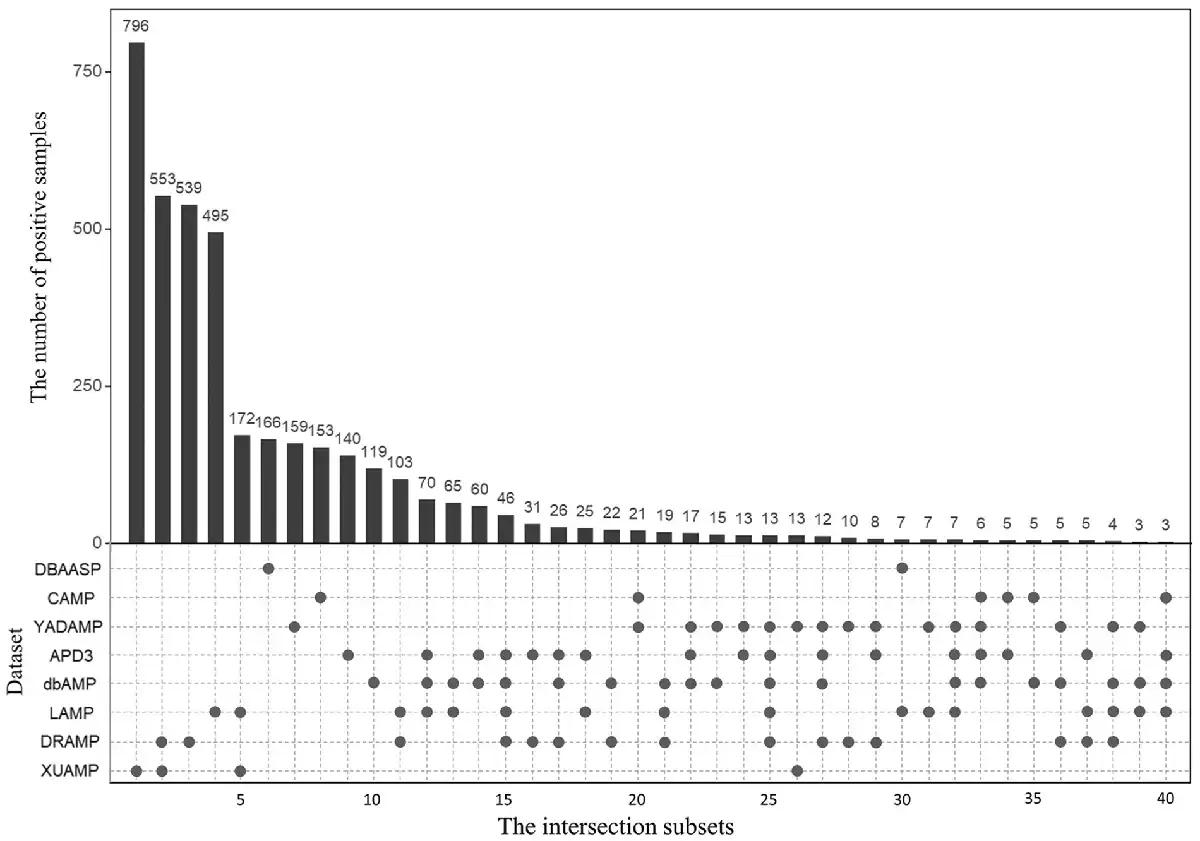
Fig. 1
The number of overlapping positive samples among the eight independent test positive datasets. There are two parts in this figure. The upper part shows the number of positive samples in each intersection subset. Only the intersection subsets with more than two positive samples are shown. The bottom part shows the detailed information of the eight independent test positive datasets, where the black spots indicate that the corresponding independent test positive datasets listed in the y-axis share the intersection subset listed in the same column in the upper part. For examples, for column 11, there are 2 black spots in the bottom part, indicating that the independent test datasets LAMP and DRAMP share the intersection subset with 103 positive samples. In other words, LAMP and DRAMP share 103 common positive samples

2.2 Benchmark datasets
In this study, we construct a pretraining dataset, and based on which a benchmark dataset is constructed. The pretraining dataset is used for pretraining the proposed method to initialize the GAT framework, and the benchmark dataset is utilized for training and predicting the proposed method. The pretraining dataset containing 5536 AMPs and 5536 non-AMPs was constructed based on SATPdb (), ADAM (), AMPfun (), APD3 (), CAMP (; ), LAMP (; ), DRAMP (), dbAMP () and databases. The sequence similarity between any two AMPs is <90%, and the sequence similarity between any two non-AMPs is <40% (). Then, a benchmark dataset is constructed to avoid the misleading model prediction caused by the length distribution gap between AMPs and non-AMPs. We selected the positive samples and negative samples with the lengths in the range of 40–100 residues from the pretraining dataset to construct the benchmark dataset. The sequence length distributions of the samples in the benchmark dataset are shown in Supplementary Figure S2.
For model training, 80% of the samples in the benchmark dataset are randomly selected as the training dataset, and the remaining 20% are used as a validation dataset to optimize the parameters. The detailed steps of the dataset construction are described in Supplementary File S1.
2.3 Overview of sAMPpred-GAT
The framework of sAMPpred-GAT is shown in Figure 2. The sAMPpred-GAT predictor extracts the residue-level features from the sequence information and the spatial relationships among the residues from the predicted structural information. Then the graphs are constructed to integrate the information of peptides, where the edges represent the structural information and the nodes represent the residue information, including sequence information and evolutionary information. Subsequently, we utilize the GAT to extract the features from the graphs-based data. Finally, we use the linear layer to predict whether a new peptide is an AMP or not.
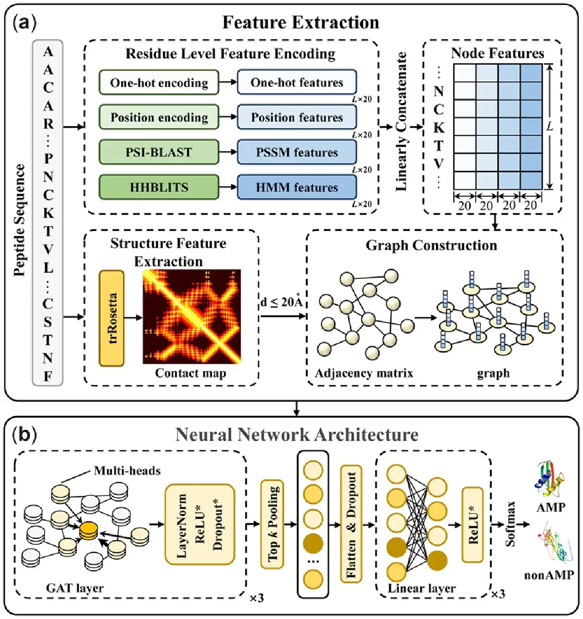
Fig. 2
The framework of sAMPpred-GAT. (a) The flowchart of feature extraction and graph construction process. For the residue-level features, we extract four different features, including one-hot features, position encoding features, PSSM features and HMM features. For structure features, we extract the contact maps by using trRosetta (). The four residue-level features represented as the nodes and the adjacency matrix information represented as the edges are fed into the GAT framework. (b) The neural network architecture of sAMPpred-GAT. We use three GAT layers with multi-head attention to capture the information from the neighbors. The GAT module utilizes both the contact map information and four residue-level features as described above, and outputs the sequence-level features in the last layer. Then we utilize the top k pooling to transform the graphs into vectors with fixed length, which is the graph level representation. The linear layers are used to make the final prediction. The methods with suffix * indicate that they are not used in the last layer
2.4 Sequence feature extraction and graph construction module
In this section, we represent the sequences from two perspectives information, including residue-level features and structural features. Specifically, the residue-level features are represented by the amino acid composition information, amino acid position information and evolutionary information. The structural information is extracted by the trRosetta (), which is converted the raw sequences into the corresponding structures, which contain the distances and orientations between all the amino acid pairs along the sequence.
2.4.1 Residual level features encoding
The proposed method utilizes four comprehensive features to represent residue-level features, including One-hot encoding features, Position encoding features, Position Specific Scoring Matrix (PSSM) features, and Hidden Markov Models (HMM) features.
One-hot encoding: to represent the composition information, we use one-hot to encode 20 standard amino acids. One-hot is a binary vector with only one position having a value of 1, representing the current acid amino, and the rest are set as 0. For example, amino acid A is coded as . The dimension of the one-hot feature is -D.
Position encoding: position encoding is claimed as an effective descriptor in many applications calculated by : where the indicates the position of the amino acid in the sequence ( ). represents the length of the peptide sequence. The variable represent each position of the vector. It can be seen from Equations (1 and 2) that the values of odd positions and even positions are distinct. The and d are constants, and their values are set to 1000 and 20 in this study, respectively. The dimension of the position encoding feature is -D.
PSSM encoding: PSSM is one of the widely used evolutionary profiles, which is generated through the multiple sequence alignment (MSA) by running PSI-BLAST() (‘-num_ iterations 3 -evalue 0.01’). The query sequence is searched by the PSI-BLAST tool through the nrdb90 database (). Because the length of AMP sequences is <100, the alignments of several peptides cannot be generated. For these peptides, their PSSMs are produced by the PSI-BLAST to search the NR database () instead of the nrdb90 database (). The dimension of the PSSM feature is -D.
HMM encoding: in this study, the HMM profile is obtained by searching the query sequence against the Uniclust30 database using HHblits () with parameters ‘-n 3 -e 0.01’. The dimension of HMM is , where the first 20 columns represent the amino acids match state frequencies, and the rest 10 columns represent seven translation frequencies and three local diversities. In this study, the first 20 columns are used as the residue-level features, which are similar to the PSSM profile (). According to the HHblits manual (), in the HMM profile is calculated by , where denotes the amino acid match state frequency. Therefore, each score is converted as ():
Finally, the residue-level features are represented by integrating four descriptors, including one-hot encoding, position encoding, PSSM encoding and HMM encoding. The dimension of the residue-level feature is -D.
2.4.2 Structure feature encoding
The study shows that the AMP sequences have low sequence homology, but the corresponding structures of the AMPs may have high similarity (,). Therefore, the structural properties are able to effectively predict the AMPs and non-AMPs. Because the peptide structures validated by the experimental method are limited, their structures are predicted by computational methods, such as trRosetta (), etc.
The trRosetta predicts the protein structures based on the predicted contact maps. The predicted contact map contains distance information and angles of all residue pairs. In this study, we utilize the distance information between pairs of atoms in contact map to represent the spatial relationship of the residues. The distance information is a binary matrix, where denotes the number of amino acids, and the element is defined as (): where is the distance between atoms and , is the threshold distance. In this study, is set as 20 Å, which is optimized on the validation dataset. The input MSA of the peptide sequence is constructed by the HHblits, and the other parameters of trRosetta are set as default values.
2.4.3 Graph construction
In this section, we utilize the graph to represent the peptide sequence, where the nodes consist of the residues-level information, and the edges are constructed according to the distance of the inter-residue pairs based on the structural information.
For discussion convenience, a graph is defined as , where is the set of nodes, and is a node feature represented by the residue-level feature with the dimension of . stands for the edge set of the graph.
2.5 Neural network architecture module
After constructing the graphs based on structural features and sequence features, a neural network based on GAT is designed to integrate information from the neighbor nodes and performs the prediction. It consists of three main modules, including (i) graph attention layers, (ii) top k pooling and (iii) output layers. The graph attention layers are utilized to extract the structural information from the graph of the sequence. The top k pooling can adaptively select the top k most informative nodes to generate the graph-level representation of the peptide. Finally, the output layers utilize the graph-level context vector to predict whether a peptide is an AMP or not.
2.5.1 Graph attention layers
In this section, we utilize the GAT () to extract the structural information from the graph constructed based on the predicted structures. It leverages masked self-attention mechanism to automatically assign weights to neighbor nodes along the edges. The larger the weight is, the more important the neighbor node is. Therefore, GAT captures the local associations between amino acids and their neighbors. In addition, GAT is robust for predicted structure data. Due to a large gap between the real pairwise distance and the predicted pairwise distance caused by the structural prediction noise, GAT can adaptively assign smaller weights to those noisy data to reduce the negative impact of noisy data on the prediction results. The process is shown in Figure 3.

Visualization of converting the process AMP structure into a complex graph. The ball and stick model in the left subfigure represent the substructure of the peptide, where the center ball represents the central amino acid atom and the other balls are the atoms of amino acids within the threshold predicted by trRosetta. The right subfigure represents the process of updating the central node features using GAT. The characters ‘K’, ‘T’, ‘V’, ‘N’, ‘P’ and ‘C’ represent the corresponding amino acids of the target atoms
Let denotes the representation of node with a dimension in the layer . is the feature of node constructed in Section 2.4. is the feature of node after the last GAT layer. The neighborhood of a node is defined as . GAT updates the node representation in an iterative way by using the following rule (): where is the projection transformation matrix in the layer . Compared with the GCN utilizing the fixed weights based on the degrees of the respective nodes, GAT aggregates the neighboring features with the self-attention-based weights. The attention coefficients is computed by (): where is a LeakyReLU activation function and is a vector of learnable parameters. represents concatenation.
Besides, multi-head attention mechanism () is used in this study for the polysemous phenomenon. GAT with heads is equivalent to integrate H single GAT layers in parallel. Moreover, except for the last layer, () and () are used after each GAT layer to enhance the ability of non-linear learning and generalization, respectively.
2.5.2 Top k pooling
Top k pooling is an module to adaptively select a certain number of nodes (). In this task, it converts the variable length amino acid sequence features into a fixed-length vector by selecting the top k residues (nodes) with the highest score.
Top k pooling computes the scalar projection score for a node with feature , which measures how much information of node reserves when projected onto the direction of a learnable vector . Then the new representation is calculated based on the indices corresponding to the top k nodes. The calculation process is as follows (): where is the vector set of projection score; is used to select the top k most informative nodes and returns their indices set . is a non-linear function and is the elementwise product.
Finally, we obtain the graph representation by concatenating them linearly:
2.5.3 Output layers
To predict whether the input sequence is an AMP or not, the linear layers are needed to learn a more discriminative representation, defined as (): where and are the input vector and output vector in the th linear layer, respectively. . denotes the weight matrix and is the bias of th linear layer. and are used following each linear layer except the last one. After the last layer, a function () is added to perform the final prediction. where denotes the binary label. Here AMP is labeled as 1, while non-AMP is labeled as 0. denotes the negative or positive probabilistic. is the total number of linear layers.
2.5.4 The model implementation
We utilized the PyTorch (https://pytorch.org/) and PyTorch Geometric () to implement sAMPpred-GAT. The negative log-likelihood loss function is used to measure the gap between predicted labels and truth labels. The ADAM algorithm () is adopted to optimize GAT with a batch size of 512 during the training process. The initial learning rate of pretraining is set as 0.001, which is decayed to 95% for every 5 epochs. A total of 50 epochs are iterated. Then a smaller learning rate of 0.0001 and fewer epochs 20 are adapted to train the model. The other parameters are the same in both the two stages. The hyperparameters are optimized based on the grid search strategy according to the maximum AUC. Please refer to Supplementary Tables S1 and S2 for more information.
2.6 Evaluation metrics
In this study, we utilize five metrics to evaluate the proposed method, which are calculated by: where TP, FP, TN and FN are the number of true positives, false positives, true negatives and false negatives, respectively (; ; ).
3 Results and discussion
3.1 Performance on XUAMP independent test dataset
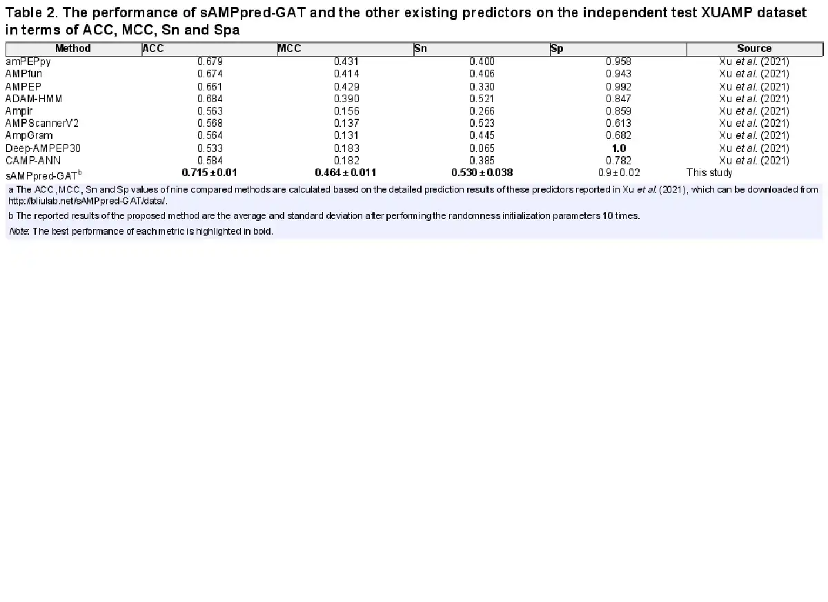
In this section, we compare the proposed method with nine state-of-the-art methods on the independent test XUAMP dataset, including amPEPpy (), AMPfun (), AMPEP (), ADAM-HMM (), ampir (), AMPScannerV2 (), AMPGram (), Deep-AMPEP30 () and CAMP-ANN (). For the sake of avoiding overestimating the performance of sAMPpred-GAT, the positive samples in the benchmark dataset sharing more than 90% similarities with any positive sample in the XUAMP independent test dataset are removed following (). The negative samples in the benchmark dataset sharing more than 40% similarities with any negative sample in the XUAMP independent test dataset are removed as well. To avoid the randomness of the initialization parameters, the proposed method sAMPpred-GAT is run 10 times with random seeds.
The experimental results of different methods are shown in Figure 4 and Table 2, from which we can observe that sAMPpred-GAT achieves the best performance in terms of AUC, ACC, MCC and Sn, and achieves highly comparable Sp. The results show that the proposed method achieves the highest AUC with fewer false positives. Therefore, sAMPpred-GAT is a useful predictor for identifying AMPs.
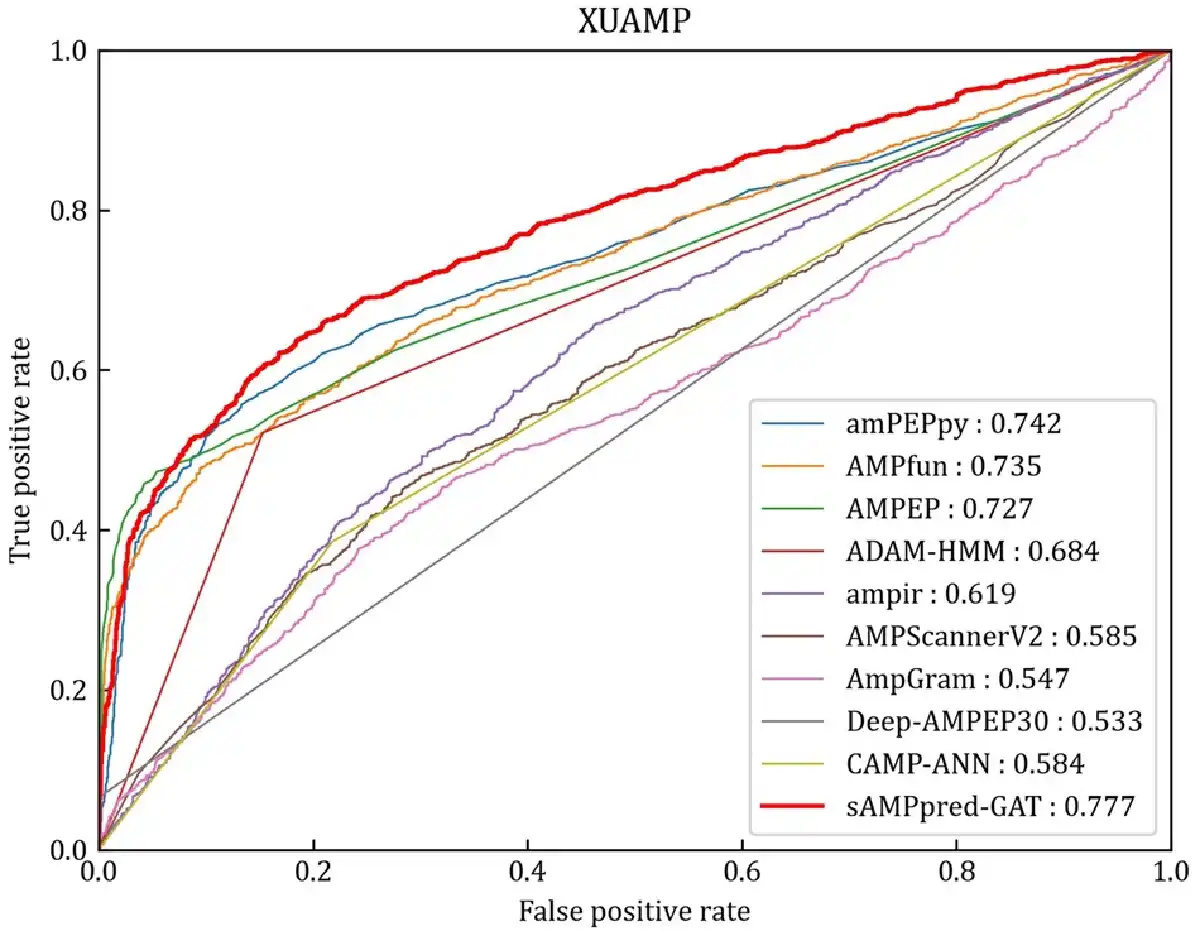
Fig. 4
ROC curves of sAMPpred-GAT and the other state-of-the-art methods on the XUAMP test dataset. The results of the other nine predictors are from
3.2 Performance on the other independent test datasets
In this section, we comprehensively evaluate the performance of sAMPpred-GAT on the seven independent test datasets, including APD3 (; ), DRAMP (; ; ), LAMP (; ; ), CAMP (; ; ), dbAMP (; ), YADAMP (; ) and DBAASP.
For the sake of avoiding overestimating the performance of sAMPpred-GAT, for each target independent test dataset, the positive samples in the benchmark dataset sharing more than 90% similarities with any positive sample in the target independent test dataset are removed following (). The negative samples in the benchmark dataset sharing more than 40% similarities with any negative sample in the target independent test dataset are removed ().
We evaluate the performance of sAMPpred-GAT and the other state-of-the-art methods on the following independent test datasets: APD3 (), DRAMP (; ), LAMP (; ), CAMP (; ), dbAMP () and YADAMP (). The results are listed in Figure 5, Supplementary Tables S3 and S4. Although sAMPpred-GAT outperforms most of the compared methods, it achieves similar performance as amPEPpy (), AMPfun () and AMPEP () on these six independent test datasets. However, we found that many samples in the six independent test datasets already exist in the corresponding training sets of amPEPpy, AMPfun and AMPEP (see Supplementary Table S5). Therefore, the performance of these three methods on the six independent test datasets would be overestimated. In order to validate this point, we removed all these overlapping samples from the six independent test datasets to make sure that there is no overlapping sample between the training sets of the three compared methods and the six independent test datasets, and then the sAMPpred-GAT, amPEPpy, AMPfun and AMPEP were re-evaluated on these six non-redundant independent test datasets (see Supplementary Tables S6–S8). From these tables, we can see that the performance of amPEPpy, AMPfun and AMPEP decreases obviously, and sAMPpred-GAT outperforms all these three compared methods. Therefore, we conclude that the performance of amPEPpy, AMPfun and AMPEP on the six independent test datasets is indeed overestimated, and sAMPpred-GAT outperforms all the compared methods. Moreover, we further evaluate the performance of sAMPpred-GAT on the independent test dataset DBAASP, and its performance is compared with amPEPpy, AMPfun and AMPEP (see Supplementary Fig. S3). The results further confirm the better of sAMPpred-GAT.
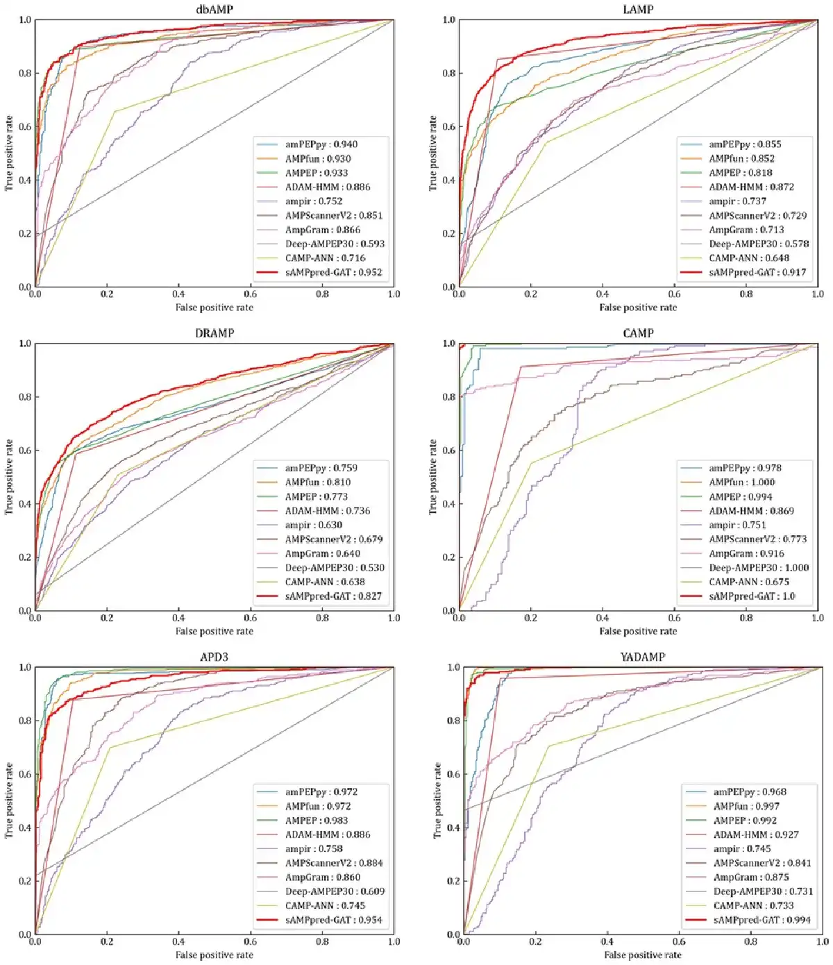
Fig. 5
ROC curves of sAMPpred-GAT and the other nine predictors on the six independent test datasets. The results of the other nine predictors are from
The sAMPpred-GAT predictor captures more discriminative features, while most of the existing methods utilized the hand-crafted features based on the experience. Therefore, the sAMPpred-GAT method is a useful tool for AMPs prediction.
3.3 Effectiveness of structural features
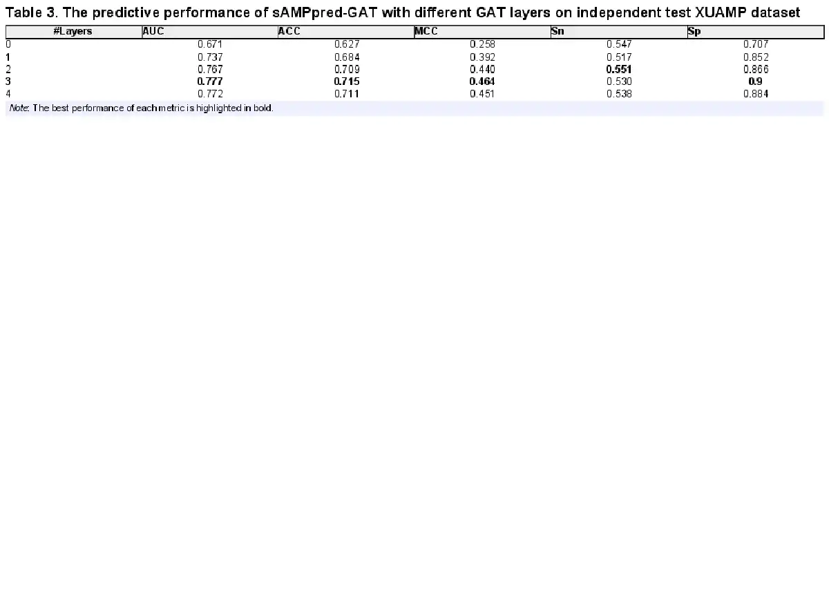
In this section, we analyze the effectiveness of structural features and the different numbers of GAT layers on the performance of sAMPpred-GAT on XUAMP dataset (see Table 3). The results show that when the number of GAT layers is set as three, which obtains the best performance in terms of AUC. The performance of sAMPpred-GAT decreases when the layer number is higher than three, caused by the problem of over-smoothing in GNNs (). Moreover, when the number of GAT layers is 0, we only utilize the residue-level sequence features. The corresponding performance of sAMPpred-GAT is low, indicating that the structural features are discriminative and can improve the predictive performance. Therefore, the proposed method utilizes the GAT framework to extract the discriminative features from the structural properties of peptides so as to improve the predictive performance.
3.4 Analysis of sequential features
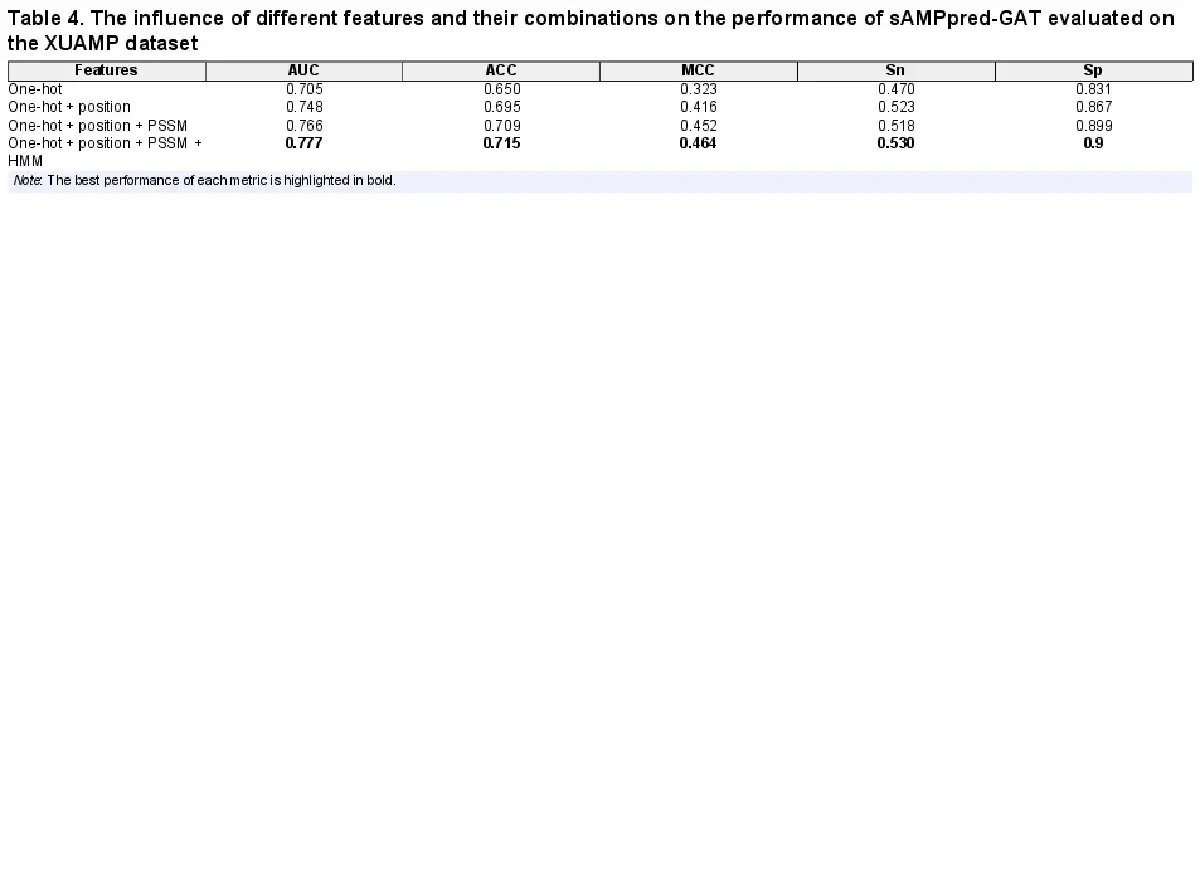
In this section, we conduct an ablation experiment to evaluate the contribution of different residue-level sequential features to the performance of the sAMPpred-GAT predictor on the independent test XUAMP dataset. The results are shown in Table 4, from which we see that when residue-level features with different properties are linearly combined, the performance of sAMPpred-GAT improves steadily. When we utilize the position encoding residue-level features, the performance of the proposed method improves obviously. Specifically, the position features improve the predictive performance by 4.3% and 4.5% in terms of AUC and ACC, respectively. The reason is that the machine learning predictors based on the GNN fail to capture the position information (; ). As a result, the features associated with the position information is able to improve the prediction performance of sAMPpred-GAT. In addition, the proposed method extracts the evolutionary information by using neural networks, which can better distinguish the AMPs. Therefore, sAMPpred-GAT accurately predicts the AMPs by integrating the position and evolution information via using the GAT.
3.5 Visualization of the features extracted by sAMPpred-GAT
The sAMPpred-GAT predictor mainly utilizes the GAT framework to automatically learn the inherent features from the structural information, sequence information and evolutionary information. To intuitively demonstrate the effectiveness of the learned features, we utilize the agglomerative clustering algorithm () to hierarchically cluster the learned features of the peptides from the XUAMP dataset. The results are shown in Figure 6, from which we can observe that: (i) the learned features with high values form the blocks, which indicates that peptides with similar functions have similar characteristics, and the peptides with different functions have different features. (ii) The peptides from the same function were groups into the same cluster. The learned features are more clearly to distinguish the AMP and non-AMP in feature space distribution. Therefore, the learned features extracted by sAMPpred-GAT are discriminative, contributing to the performance of sAMPpred-GAT for predicting AMPs.
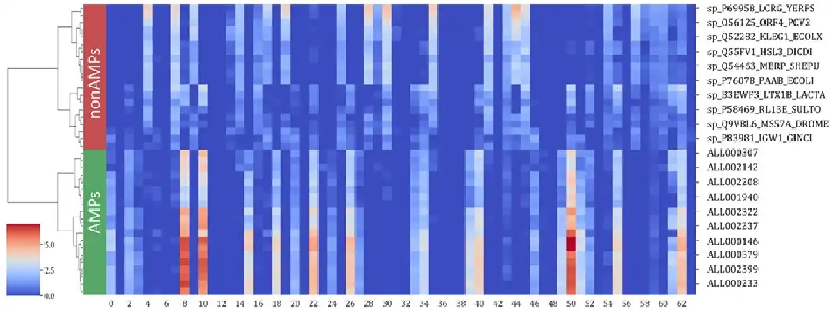
Fig. 6
Analysis of the learned features extracted by the sAMPpred-GAT by running agglomerative clustering over 40 peptides from XUAMP dataset. The learned features are extracted from the penultimate full connection layer with 64-D
4 Conclusion
AMPs are essential biomolecules of therapeutic peptides for the immune system of organisms. In this study, we proposed a sAMPpred-GAT predictor based on the predicted peptide structure information for AMPs recognition. The proposed method utilizes structural information, evolutionary profiles and sequence features to construct the graphs. Then the proposed method extracts the discriminative features from the graph by using the GAT framework. Finally, the optimized features are fed into the output layer to predict the AMPs. Experimental results show that the sAMPpred-GAT outperforms the other state-of-the-art methods in terms of AUC, and achieves better or highly comparable performance in terms of the other metrics on the eight independent test datasets. The framework using structural features and GAT layers can learn the inherent features with more discriminative power so as to improve the predictive performance. The GAT would have many other potential applications in bioinformatics, such as non-coding RNA and disease association identification, peptide prediction, etc.
Acknowledgments
The authors were very much indebted to the three anonymous reviewers, whose constructive comments are very helpful for strengthening the presentation of this article.
Funding
This work was supported by the National Natural Science Foundation of China [62102030, U22A2039 and 62271049] and the Beijing Natural Science Foundation [JQ19019].
Conflict of Interest: none declared.
References
- Altschul S.F. et al (1997) Gapped BLAST and PSI-BLAST: a new generation of protein database search programs. Nucleic Acids Res., 25, 3389–3402.
- Bahar A.A., Ren D. (2013) Antimicrobial peptides. Pharmaceuticals (Basel), 6, 1543–1575.
- Barreto-Santamaria A. et al (2019) Designing and optimizing new antimicrobial peptides: all targets are not the same. Crit. Rev. Clin. Lab. Sci., 56, 351–373.
- Bhadra P. et al (2018) AmPEP: sequence-based prediction of antimicrobial peptides using distribution patterns of amino acid properties and random Forest. Sci. Rep., 8, 1697.
- Burdukiewicz M. et al (2020) Proteomic screening for prediction and design of antimicrobial peptides with AmpGram. Int. J. Mol. Sci., 21, 4310.
- Charoenkwan P. et al (2021) StackIL6: a stacking ensemble model for improving the prediction of IL-6 inducing peptides. Brief. Bioinform., 22, bbab172.
- Chen D. et al (2020) Measuring and relieving the over-smoothing problem for graph neural networks from the topological view. Proc. AAAI Conf. Artif. Intell., 34, 3438–3445.
- Chen J., Shi X. (2019) Sparse convolutional denoising autoencoders for genotype imputation. Genes (Basel), 10, 652.
- Chen J. et al (2021) PAR-GAN: improving the generalization of generative adversarial networks against membership inference attacks. In: Proceedings of the 27th ACM SIGKDD Conference on Knowledge Discovery & Data Mining, Virtual Event, Singapore. Vol. 11, 127–137.
- Chung C.-R. et al (2020) Characterization and identification of antimicrobial peptides with different functional activities. Brief. Bioinform., 21, 1098–1114.
- de la Fuente-Nunez C. et al (2017) Antimicrobial peptides: role in human disease and potential as immunotherapies. Pharmacol. Ther., 178, 132–140.
- Fan L. et al (2016) DRAMP: a comprehensive data repository of antimicrobial peptides. Sci. Rep., 6, 24482.
- Fey M., Lenssen J. (2019) Fast Graph Representation Learning with PyTorch Geometric.arXiv preprint arXiv:1903.02428.
- Fingerhut L. et al (2021) Ampir: an R package for fast genome-wide prediction of antimicrobial peptides. Bioinformatics, 36, 5262–5263.
- Gao H., Ji S. (2019) Graph u-nets. In: International Conference on Machine Learning. PMLR. pp. 2083–2092.
- Gaspar D. et al (2013) From antimicrobial to anticancer peptides. Front. Microbiol., 4, 294.
- Gligorijević V. et al (2021) Structure-based protein function prediction using graph convolutional networks. Nat. Commun., 12, 3168.
- Goodfellow I. et al (2016) Deep Learning. MIT Press, Cambridge, MA, USA.
- Guo Y. et al (2021) PreTP-EL: prediction of therapeutic peptides based on ensemble learning. Brief. Bioinform., 22, bbab358.
- Holm L., Sander C.J.B. (1998) Removing near-neighbour redundancy from large protein sequence collections. Bioinformatics, 14, 423–429.
- Huang Y. et al (2010) CD-HIT suite: a web server for clustering and comparing biological sequences. Bioinformatics, 26, 680–682.
- Jenssen H. et al (2006) Peptide antimicrobial agents. Clin. Microbiol. Rev., 19, 491–511.
- Jhong J.H. et al (2019) dbAMP: an integrated resource for exploring antimicrobial peptides with functional activities and physicochemical properties on transcriptome and proteome data. Nucleic Acids Res., 47, D285–D297.
- Jhong J.-H. et al (2022) dbAMP 2.0: updated resource for antimicrobial peptides with an enhanced scanning method for genomic and proteomic data. Nucleic Acids Res., 50, D460–D470.
- Jin Q. et al (2020) RA-UNet: a hybrid deep attention-aware network to extract liver and tumor in CT scans. Front. Bioeng. Biotechnol., 8, 605132.
- Jumper J. et al (2021) Highly accurate protein structure prediction with AlphaFold. Nature, 596, 583–589.
- Kang X. et al (2019) DRAMP 2.0, an updated data repository of antimicrobial peptides. Sci. Data, 6, 148.
- Kingma D.P., Ba J.J. (2014) Adam: A Method for Stochastic Optimization. In: Proceedings of the 3rd International Conference on Learning Representations (ICLR), San Diego, CA.
- Lai B., Xu J. (2022) Accurate protein function prediction via graph attention networks with predicted structure information. Brief. Bioinform., 23, bbab502.
- Lawrence T.J. et al (2021) amPEPpy 1.0: a portable and accurate antimicrobial peptide prediction tool. Bioinformatics, 37, 2058–2060.
- Lee H.T. et al (2015) A large-scale structural classification of antimicrobial peptides. Biomed Res. Int., 2015, 475062.
- Li C. et al (2022) AMPlify: attentive deep learning model for discovery of novel antimicrobial peptides effective against WHO priority pathogens. BMC Genomics, 23, 1–15.
- Liu Y. et al (2020) Deep learning of high-order interactions for protein interface prediction. In: Proceedings of the 26th ACM SIGKDD International Conference on Knowledge Discovery & Data Mining, pp. 679–687.
- Nair V., Hinton G.E. (2010) Rectified linear units improve restricted boltzmann machines. In: ICML.
- O'Leary N.A. et al (2016) Reference sequence (RefSeq) database at NCBI: current status, taxonomic expansion, and functional annotation. Nucleic Acids Res., 44, D733–D745.
- Pang Y. et al (2021) Identifying anti-coronavirus peptides by incorporating different negative datasets and imbalanced learning strategies. Brief. Bioinform., 22, 1085–1095.
- Piotto S.P. et al (2012) YADAMP: yet another database of antimicrobial peptides. Int. J. Antimicrob. Agents, 39, 346–351.
- Pirtskhalava M. et al (2021) DBAASP v3: database of antimicrobial/cytotoxic activity and structure of peptides as a resource for development of new therapeutics. Nucleic Acids Res., 49, D288–D297.
- Remmert M. et al (2012) HHblits: lightning-fast iterative protein sequence searching by HMM-HMM alignment. 9, 173–175.
- Rokach L., Maimon O. (2005) Clustering methods. In: Data Mining and Knowledge Discovery Handbook, pp. 321–352. Springer.
- Saxena S., Gomber C. (2010) Surmounting antimicrobial resistance in the millennium superbug: staphylococcus aureus. Open Med., 5, 12–29.
- Shi G. et al (2022) DRAMP 3.0: an enhanced comprehensive data repository of antimicrobial peptides. Nucleic Acids Res., 50, D488–D496.
- Singh S. et al (2016) SATPdb: a database of structurally annotated therapeutic peptides. Nucleic Acids Res., 44, D1119–1126.
- Song J. et al (2019) iProt-Sub: a comprehensive package for accurately mapping and predicting protease-specific substrates and cleavage sites. Brief. Bioinform., 20, 638–658.
- Srivastava N. et al (2014) Dropout: a simple way to prevent neural networks from overfitting. BibSonomy, 15, 1929–1958.
- Thakur N. et al (2012) AVPpred: collection and prediction of highly effective antiviral peptides. Nucleic Acids Res., 40, W199–W204.
- Thomas S. et al (2010) CAMP: a useful resource for research on antimicrobial peptides. Nucleic Acids Res., 38, D774–D780.
- UniProt Consortium. (2015) UniProt: a hub for protein information. Nucleic Acids Res., 43, D204–D212.
- Vaswani A. et al (2017) Attention is all you need. Adv. Neural Inf. Process. Syst., 30, 5998–6008.
- Veličković P. et al (2017) Graph Attention Networks.
- Veltri D. et al (2018) Deep learning improves antimicrobial peptide recognition. Bioinformatics, 34, 2740–2747.
- Waghu F.H. et al (2016) CAMPR3: a database on sequences, structures and signatures of antimicrobial peptides. Nucleic Acids Res., 44, D1094–1097.
- Wang G. et al (2016) APD3: the antimicrobial peptide database as a tool for research and education. Nucleic Acids Res., 44, D1087–1093.
- Wang Z., Wang G. (2004) APD: the antimicrobial peptide database, Nucleic Acids Res., 32, D590–D592.
- Wei L. et al (2018) ACPred-FL: a sequence-based predictor using effective feature representation to improve the prediction of anti-cancer peptides. Bioinformatics, 34, 4007–4016.
- Wei G.-W. (2019) Protein structure prediction beyond AlphaFold. Nat. Mach. Intell., 1, 336–337.
- Wei L. et al (2021a) Computational prediction and interpretation of cell-specific replication origin sites from multiple eukaryotes by exploiting stacking framework. Brief. Bioinform., 22, bbaa275.
- Wei L. et al (2021b) ATSE: a peptide toxicity predictor by exploiting structural and evolutionary information based on graph neural network and attention mechanism. Brief. Bioinform., 22, bbab041.
- Xia Y. et al (2021) GraphBind: protein structural context embedded rules learned by hierarchical graph neural networks for recognizing nucleic-acid-binding residues. Nucleic Acids Res., 49, e51.
- Xu J. et al (2021) Comprehensive assessment of machine learning-based methods for predicting antimicrobial peptides. Brief. Bioinform., 22, bbab08.
- Yan J. et al (2020) Deep-AmPEP30: improve short antimicrobial peptides prediction with deep learning. Mol. Ther. Nucleic Acids, 20, 882–894.
- Yan K. et al (2019) Protein fold recognition based on multi-view modeling. Bioinformatics, 35, 2982–2990.
- Yan K. et al (2022a) TPpred-ATMV: therapeutic peptides prediction by adaptive multi-view tensor learning model. Bioinformatics, 38, 2712–2718.
- Yan K. et al (2022b) TP-MV: therapeutic peptides prediction by multi-view learning. Curr. Bioinform., 17, 174–183.
- Yang J. et al (2020) Improved protein structure prediction using predicted interresidue orientations. Proc. Natl. Acad. Sci. USA, 117, 1496–1503.
- Ye G. et al (2020) LAMP2: a major update of the database linking antimicrobial peptides. Database (Oxford), 2020, baaa061.
- You J. et al (2019) Position-aware graph neural networks. In: International Conference on Machine Learning, pp. 7134–7143. PMLR.
- Zasloff M. (2002) Antimicrobial peptides of multicellular organisms. Nature, 415, 389–395.
- Zhao T. et al (2021) Identifying drug-target interactions based on graph convolutional network and deep neural network. Brief. Bioinform., 22, 2141–2150.
- Zhao X. et al (2013) LAMP: a database linking antimicrobial peptides. PLoS One, 8, e66557.