Introduction
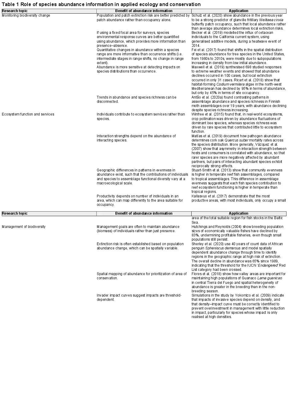
Environmental change alters the occurrence and local abundance patterns of species (Antão et al. , Hastings et al. , Lenoir et al. , Román‐Palacios and Wiens ). Modelling species occurrence has helped predict the distribution and erosion of biodiversity under unprecedented rates of environmental change (Pereira et al. , Kissling et al. , Jetz et al. ). Species occurrence models, however, provide limited opportunities to understand local abundance changes that accompany species distribution shifts (Lenoir and Svenning , Bates et al. , Hastings et al. ). Species present in high numbers at only a few sites can make large contributions to ecological processes, but a focus on occurrence would overlook these species (Table 1; Stuart‐Smith et al. , Williams et al. , Johnston et al. , Winfree et al. , Genung et al. ). Abundance trends can also act as an early warning signal of population collapse (Clements et al. , Ceballos et al. ), but occurrence patterns may not change until after local population depletion (Hastings et al. ). To better inform spatial conservation planning, we must better monitor and predict species abundance (Margules and Pressey , Pauly and Froese , Mi et al. ). However, abundance‐based species distribution models remain underdeveloped relative to occurrence‐based models.
As in occurrence‐based models, modelling abundance according to abiotic environmental conditions depends on assumptions of niche theory (Maguire , Holt ). Critically, environmental conditions are assumed to affect demographic processes which in turn drive population dynamics (Maguire , Brown et al. , Holt , Pearce‐Higgins et al. , Betts et al. ). For a given species, spatial abundance variation is a consequence of these links coupled with natural environmental gradients (Holt ). If this theory is accurate, predictions of local abundance from environmental factors should be possible (Maguire , Martínez‐Meyer et al. , Waldock et al. ).
Yet, abundance does not appear to always be strongly constrained by theoretical niche properties in empirical data (Yañez‐Arenas et al. , Dallas et al. , Osorio‐Olvera et al. , Santini et al. , Dallas and Santini , Holt , Sporbert et al. ). For example, Allee effects, non‐equilibrium population states, demographic stochasticity and environmental variability act to weaken the link between environmental conditions and local abundance (Osorio‐Olvera et al. , Dallas and Santini , Holt ). If these factors dominate over macro‐environmental constraints on abundance, then abundance will be poorly predicted using a species distribution modelling approach. Additionally, it is not clear whether there is always a strong linear link between predicted habitat suitability, or occurrence probability, and species local abundance (Vanderwal et al. , Dallas and Hastings ). If indirectly predicting abundance from habitat suitability is ineffective, this demands us to explore more directly predicting abundance using species distribution models. At present, the expected predictive power when modelling abundance in relation to environmental conditions is poorly understood and not quantitatively reviewed over large datasets and a varied set of modelling frameworks.
Recent decades of statistical algorithm development provide an opportunity to evaluate the performance of abundance‐based species distribution models. Current abundance model evaluations examine only a limited set of statistical frameworks, and the best options may be overlooked (Pearce and Ferrier , Potts and Elith , Oppel et al. , Bahn and McGill ). For example, if abundance is determined by nonlinear and complex interactions of environmental factors, then machine‐learning algorithms may be most appropriate (Merow et al. , Zurell et al. ). In contrast, simpler models may be favoured if species environmental responses closely follow simple unimodal functions (Austin , Ready et al. , Boucher‐Lalonde et al. , Waldock et al. ). Simpler models are also expected to perform better when extrapolated to new environmental conditions (Merow et al. , Brun et al. ).
Species distribution model performance is often associated with species and data characteristics. Establishing how and why model performance varies for different species is critical for conservation and management applications, particularly with respect to commonness and rarity. Common species, in terms of local and regional abundance, often contribute most to ecosystem functioning (Genung et al. ). Low abundance and range‐restricted species may be prioritised for conservation, having higher extinction risk (Purvis et al. , Ceballos et al. ) and potentially playing unique roles in ecosystems (Violle et al. ). Species distribution models generally perform better for species with smaller ranges, lower endemicity and non‐migratory behaviour; in addition, the number of observations positively affects performance (McPherson and Jetz , Newbold et al. , Chefaoui et al. , Thuiller et al. ).
The influence of species characteristics on abundance model performance is less well established. For certain species, such as those with large and well‐occupied ranges, it could be challenging to model abundance accurately because theory predicts for these species environmental niches play a smaller role in controlling abundance (Chisholm and Muller‐Landau , Peterson et al. , Yañez‐Arenas et al. , Chu et al. , Bowler et al. , Yenni et al. , Hallett et al. ). In contrast, rare (low mean abundance) species that have narrow niches often exhibit more stable populations and therefore abundance could be more predictable (Yenni et al. ). Additionally, data characteristics could affect the success of species distribution model performance. More samples generally improve species distribution model performance by being less geographically and environmentally biased (Wisz et al. ) and should similarly improve abundance model performance (Yañez‐Arenas et al. ). Yet, these effects have not been tested.
Here, we aim to provide practical guidance on applying statistical approaches to predict species abundance and identify factors most affecting predictive performance. We compare 68 abundance‐based species distribution models fitted for two standardised abundance datasets containing more than 800 marine and terrestrial vertebrate species and over 800 000 abundance observations. We test model interpolative (within‐sample) and extrapolative (out‐of‐sample) performance. We ask how statistical framework and model complexity, and species and data characteristics, affect metrics of model accuracy, discrimination and precision. We show that abundance‐based species distribution models have great potential – additional to occurrence‐based models – to generate insights in spatial ecology and biogeography and to improve systematic conservation planning outcomes.
Material and methods
Spatial abundance data
We obtained standardised estimates of species abundance across large regions for birds and shallow‐water reef fishes from the Breeding Bird Survey of the USA (BBS) and Reef Life Survey (RLS), respectively (for detailed sampling schemes, see Pardieck et al. for birds and Edgar and Stuart‐Smith for fishes). For birds, abundance data comprise of 3‐min counts of individuals sighted and heard within a 400‐m stop radius along a transect of 50 stops. We summed bird species abundance across 50 stops within a sampled year and mean‐averaged abundances for a given species in a repeated site across the years 2014–2018. We aggregated abundances across years to better generalise our results to the structure of most abundance datasets, whereby yearly values across broad geographic regions are unlikely to be available (see the Supporting information for exploration of this assumption). We filtered out all samples that did not meet BBS‐established weather, date, time, route completion, randomised sampling and sampling protocol criteria (i.e. using BBS data with a run type of 1). For fishes, abundance data are counts of individuals sighted along 50‐m‐long underwater transects (summed across 2 × 5‐m‐wide blocks on either side of the transect line). We mean‐averaged RLS abundance estimates across multiple transects within sites, with sites defined as sets of transects <200 m apart (Edgar and Stuart‐Smith , Cresswell et al. ). As such, where sites are surveyed in multiple years, abundances were mean‐averaged. We filtered sites geographically between 3°S to 50°S and 110°E to 165°E to select for Australian and Indo‐Pacific survey locations where sampling effort was most intensive and comprehensive in the RLS dataset. For both BBS and RLS datasets, we removed species without full scientific names and fewer than 50 abundance records. We required species absences for two‐stage models and abundance–absence models. We generated absences for each species by taking observations where species were present and finding all observations within a 1000‐km buffer where species were not present. A lack of observed presence is not necessarily a ‘true absence' but instead suggests species were undetectable with a reasonable sampling effort (Guillera‐Arroita ). We analysed a total of 264 474 observations of 385 species in 3890 sites for birds in the BBS dataset and 567 669 observations of 495 species in 2137 sites for reef fishes in the RLS dataset.
Covariates
We matched site locations to gridded environmental variables representing climate, biogeochemistry, land‐use, depth, habitat area and human populations, retaining only variables with expected a priori relationships with abundance (see the Supporting information for details). Because of the high number of similar climate‐related variables, and to avoid multicollinearity in these, we first applied robust principal component analysis (PCA) using package pcaMethods(ver. 1.76.0; Stacklies et al. ) which is shown to be a good approach to reduce multicollinearity in species distribution models (SDM) (Cruz‐Cárdenas et al. , De Marco and Nóbrega , Osorio‐Olvera et al. ). Furthermore, we focused on predictive power to ensure our results were more robust to potential multicollinearity. We ran a separate robust PCA on 19 variables characterising climates across the bird survey locations (bio1–bio19) and on 15 variables characterising climatic and biogeochemical properties across the fish survey locations (mean, minimum and maximum of pH, salinity, chl‐a, net primary productivity, degree heating weeks; indicated in the Supporting information). For each dataset, we retained three principal components, explaining 87.8% and 77.8% variation, respectively, and used these principal component scores as predictor variables to summarise the dominant climate and biogeochemical regimes of the data in each set of models (three PCA variables for birds and three PCA variables for fishes; Supporting information). In addition to the climatological variables, we also included additional environmental variables as predictors in our model that we expected to act independently. All non‐PCA variables were mean‐centred, normalised to a variance of 1 and transformed according to the Supporting information before modelling.
Analytical design
We analysed a large diversity of species abundance models that spanned a gradient in model complexity and different formulations of abundance data. Further, we assessed model performance for interpolation and extrapolation of cross‐validation scenarios (Fig. 1). Given that data requirements are a major challenge in fitting species abundance models, we chose species‐level statistical models that were suitable for our goal of comparing predictive performance (i.e. not mechanistic, hierarchical or multispecies/joint/multivariate SDMs). In total, we fitted and evaluated 68 types of species abundance model (24 model frameworks by 3 response variable (abundance) formulations, less 4 models of zero‐inflation that are not valid for abundance‐only models = 68 models; see Supporting information for full model list). Combining models and cross‐validations for 1547 species led to 59 840 models to evaluate.

Figure 1
Overview of analysis from data sources to model performance evaluations. Model evaluation metrics for accuracy, discrimination and precision are presented.
Our full species abundance model set comprises different statistical algorithms, response transformations, error distributions and formulations of abundance data. We used 24 model variants from common statistical distributions and transformations for abundance data that were available within statistical software packages in R (e.g. Poisson, negative binomial, zero‐inflated, Tweedie, multi‐nominal, log10‐Gaussian, log‐Gaussian; Supporting information). We chose statistical treatments of abundance data that are common in the literature and valid to the error distribution of abundance. We fitted these 24 model variants using four statistical model fitting procedures: generalised linear models (GLMs), generalised additive models (GAMs; Wood 2011), gradient boosting machine (GBM; Friedman ) and random forests (RF; Breiman ). This model set varied in complexity of the relationship between abundance and environmental variables (linear to highly complex) and the behaviour of interactions within the models (none to many; Merow et al. ). For GLMs and GAMs, we used a range of error distributions rather than determining a priori the most appropriate error distribution for each species. This follows previous species abundance model comparisons (Potts and Elith ), which assumed that incorrect model specification leads to poor predictive ability, and we focused our comparison of model performance on predictive ability (which also provided standardised assessment criteria across statistical algorithms). For all models, we included the same initial set of predictor variables, although each model framework had a different underlying variable selection procedure that identified independent sets of final predictors. The full model fitting procedure, algorithm parameters and justification for each modelling approach and software used are provided in the Supporting information.
In addition to model variants, we used three formulations of response data: abundance‐when‐present (for 20 model variants, less 4 zero‐inflated models), abundance–absence (for 24 model variants) and an indirect two‐stage modelling approach (for 24 model variants). For abundance‐when‐present models, we removed all absences. Abundance–absence models were analogous to classic presence–absence data in species distribution models but using abundance estimates instead of presences. In abundance–absence models, we standardised prevalence (the number of absences compared to presences) across species, which can influence the estimation of response curves from data characteristics alone when there are many more absences than presences (Meynard et al. ). To do so, we bootstrap‐subsampled the number of absences to be twice the number of presences, repeating this procedure 10 times and averaging abundance predictions across bootstraps. Finally, our indirect two‐stage modelling approach first modelled habitat suitability as a traditional SDM by converting abundance–absences into presence–absences. Next, we used the habitat suitability predictions from this model as a single covariate to predict abundance. Note, this is not a hurdle approach but instead tests the assumption that habitat suitability correlates to, and predicts, local abundance (Vanderwal et al. ). Details for fitting SDMs to produce occupancy predictions are provided in the Supporting information.
Model evaluation: accuracy, discrimination and precision
We evaluated the consistency between predicted and observed abundance using metrics of: 1) accuracy; 2) discrimination and 3) precision (see Fig. 1 for equations; Norberg et al. ). Accuracy is the degree of proximity to a known truth, measured here using mean absolute error between observed and predicted abundance, expressed as a proportional error by dividing the mean absolute error by the mean observed abundance for a species (Amae). Discrimination measures how well model predictions discern low values from high values of observed abundance, e.g. in the correct overall ordering of abundances. This is a continuous analogue of occurrence SDMs discerning between present and absent. We measured discrimination using both Spearman's rank correlation (DSpearman) and Pearson's correlation (DPearson) between predicted and observed abundance. In addition, we estimated the slope and intercept of a linear model between predicted and observed abundance (Dslope, Dintercept). Precision measures the information content in the predictions as the variation in predicted abundance relative to the variation in the observed abundances. Precision differs from accuracy because estimates can be precise with high information content even if overall predictions were biased. Here, we measured precision as the SD of the predicted abundances (Norberg et al. ). However, we compared this value to a reasonable expectation of precision because each species has a different range of abundance values. Therefore, we estimated the SD of predicted abundance and divided this by the SD of observed abundance and call this property Pdispersion.
Accuracy, discrimination and precision capture different facets of model performance and so could be considered together or separately depending on the purposes of the modelling exercise. For example, a model can predict mean abundance of a species well (high accuracy) but poorly discriminate between high and low abundances (low discrimination). We focused our results mostly on discrimination because identifying changes in spatial and temporal variation in abundance, a goal of conservation and wildlife management, depends on good discrimination of abundance values between sites or time periods. Further, accuracy and precision may depend on the quality of sampling, but inaccurate sampling may still provide reasonable estimates of spatial and temporal differences in abundance. We identified an ‘optimal model' based on the most discriminatory model for each species. To do so, we rescaled the four discrimination metrics between 0 and 1, averaged the score across the scaled metrics and identified the model with the highest average score per species – we report this as the ‘optimal model' throughout.
Note that we avoid confounding performance in predicting presence–absences from performance in predicting abundance by only evaluating predictions for species abundances when present (i.e. we exclude any abundance values predicted in sites where species are absent in the observed data). Although many reviews exist identifying the best occupancy‐based frameworks for predicting presence or absences (Norberg et al. ), our novel contribution focuses on predicting species abundance. In practice, to obtain abundance estimates, both occupancy and abundance predictions should be combined (Denes et al. ).
We assessed whether a rescaling correction could improve the biases in abundance predictions between predicted and observed abundance. This bias appears systematically in quantitative ecological predictions (Pearce and Ferrier , Fukaya et al. , Ploton et al. ). We rescaled predicted values to take the range of observed values using the following formula
and assessed how this procedure affected model performance indicated by our evaluation metric set.
Model cross‐validations and transferability to novel climates
We evaluated model performance using two cross‐validation strategies. We evaluated how well models predict abundance when 1) interpolating within environments (within‐sample) and 2) extrapolating into novel climate conditions (out‐of‐sample). The first scenario applies when models are interpolated to fill geographic gaps in sampling within a species range. The second scenario applies, for example, when modelling species abundance under climate change. When testing interpolation within sample environments, we randomly held out 20% of the abundance data and fitted models to the remaining 80%. This within‐sample model evaluation used a random subset of sites within the full covariate space.
Our second cross‐validation strategy tested model transferability in novel conditions. Transferability measures if models can be projected beyond environments found within bounds of the covariate data. Given the rate of anthropogenic environmental change, models will be best applied when they are also accurate in novel conditions with no past analogues (Evans , Sequeira et al. ). Model transferability can be low if models are overfitted, exhibit non‐stationarity or are missing important covariates (Yates et al. ). We built separate models following the above protocol to test model transferability. To do so, we non‐randomly sampled 20% data from above the 80th quantile of sea‐surface temperature in reef fishes and above the 80th quantile of the climatological PCA‐1 in birds and fitted our abundance models to the remaining 80%. We estimated all evaluation metrics within the out‐of‐sample cross‐validation sets as above. In both scenarios, we assumed that cross‐validation frames were independent of the training data frames (Randin et al. , Roberts et al. ).
We did not perform k‐fold cross‐validation for the full span of covariate space because we wanted to gain an understanding of abundance estimates from directional environmental novelty due to climate change (e.g. predicting abundance in warmer temperatures than that fishes currently experience in the oceans). As a hypothetical example, if we split a temperature gradient from 20 to 30°C into 20–22, 22–24, 24–26, 26–28 and 28–30°C bins and examined performance on each bin, spatial autocorrelation would lead to an underestimate of model performance in novel future climates when evaluating the middle bins. Under temperature warming, we therefore only used the highest 20% bin threshold for exploring extrapolation (i.e. transferability to novel climates). To ensure cross‐validation scenarios of interpolation and extrapolation were comparable, we used only one 20% subsample for the interpolation (random) subset also. Although this procedure is not encouraged in general for SDM fitting and evaluation, for good reason (Roberts et al. ), it suits our specific cross‐validation goals (Sequeira et al. , Yates et al. ). We expected our findings to be robust to any small biases introduced by only performing one‐fold cross‐validations because of the high number of species included in the exercise. We did, however, perform 10‐fold cross‐validations when sub‐sampling species absences to ensure findings were robust to variation in the locations of species absences.
Species and data characteristics
We tested how characteristics of species abundance, frequency and data availability affected model performance. To explain variation in model performance among species, we calculated 1) the mean abundance of species when present; 2) the proportion of presence compared to absence records (within 1000 km of presence records) in the observational data (% occupied sites) and 3) the total number of presence records per species (overall observation number). Although the frequency of occurrence and the total number of presences are collinear in bird and fish datasets (rho = 0.87, rho = 0.67, respectively), we included both because unbiased estimates of coefficients are achieved through multiple regression (Morrissey and Ruxton ). We log10 transformed and standardised predictor variables to have unit variance and removed outliers (points > 2 SD from the mean) from the response variables. Next, we fitted multiple regressions that explained how the model evaluation metrics depended on our three measures of species characteristics. For simplicity, we present these results using DSpearman due to the high number of comparisons and the importance of model discrimination highlighted above. We first fitted a full model, including three two‐way interactions between pairs of predictors. We performed backwards stepwise model selection and selected the model with the lowest Akakike information criterion (AIC) score using the R package MuMIn (Burnham and Anderson , Barton ). We plotted marginal effects by predicting model effects for a given variable across the mean value of all other model covariates. We fitted these models using phylogenetic generalised least squares using the R package caper using maximum likelihood to estimate Pagel's λ (Blomberg and Symonds , Orme et al. ). We used published bird (Jetz et al. , ; <https://birdtree.org/downloads/>) and fish (Rabosky et al. ; <https://fishtreeoflife.org/downloads/>) phylogenetic trees.
Results
Overview of model performance
We first assessed performance by applying all frameworks to all species and evaluating interpolative prediction of within‐sample observations. Doing so, model performance was highly variable and generally low (Supporting information). For example, across all models and species, DSpearman had a median of 0.29 (5th percentile = −0.17, 95th percentile = 0.64), median Dslope was 0.06 (−0.07 to 0.47) and median Amae was 0.74 (0.48–1.52). As such, of the complete model set (n = 68), only 51% of species had at least one model with a DSpearman above 0.5; 53% of species had at least one model with a Dslope between 0.5 and 1.5, and 29% of species had at least one model with Amae predicting mean abundances within 50% of observed mean abundances. Overall, 13% of species had models fitting all the above criteria.
We next investigated the best‐fitting algorithm for each species independently, keeping only the single best model for each species (i.e. our ‘optimal model'). Random forests were most often selected as the optimal models for discrimination (precision, accuracy) being best for 51% (55%, 44%) of the species, gradient boosting machines for 22% (26%, 21%) and generalised linear models and generalised additive models for 16% (9%, 23%) and 12% (10%, 13%) of species, respectively (Fig. 2). Building models using abundance–absence data led to the best discrimination (precision, accuracy) performance for 68% (30%, 36%) of species, 19% (24%, 51%) using only species abundance and 14% (46%, 14%) using a two‐step indirect approach relating abundance to occurrence probability (Supporting information).
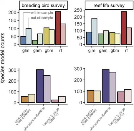
Figure 2
Counts of the model framework (top row) and abundance response treatment (bottom row) to which the most discriminatory model for each species belongs. Breeding Bird Survey is shown in the left panels, and Reef Life Survey in the right panels. Colour shading indicates whether model predictions were from the within‐sample model runs (dark) or out‐of‐sample model runs (light). See the Supporting information for counts using most accurate and most precise models, as well as combining all metric groups.
When selecting an optimal model for each species, model performance was good for most metrics (Fig. 3, Table 2). For example, there were positive correlations for most species between observed and predicted abundances, and the error of average abundance estimation was relatively low. Specifically, median DSpearman was 0.48 (0.14–0.72) and 0.43 (0.17–0.72) for bird and fish surveys, respectively, and median Amae was 0.62 (0.43–0.97) and 0.69 (0.46–1.34), respectively. Some measures of model performance were poor, leading to a biased relationship between observed and predicted abundances and a poor estimation of abundance variation. Specifically, Dslope was 0.25 (0.02–0.68) and 0.20 (0.01–0.99) for bird and fish surveys, and Pdispersion was 0.51 (0.12–1.27) and 0.44 (0.05–1.67), respectively.
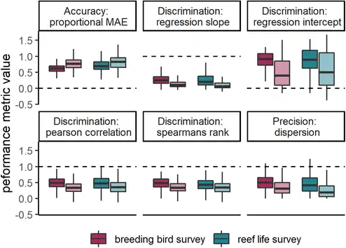
Figure 3
Box plots of model performance of most discriminatory model for each species across all six metrics. Colours indicate Breeding Bird Survey and Reef Life Survey, whereas shading indicates within‐sample and out‐of‐sample cross‐validations. Dashed lines indicate target values for each metric. Note that the type of model is not necessarily the same for a given species in the within‐sample and out‐of‐sample comparisons, as indicated in Fig. 2. Central lines correspond to median values, hinges correspond to 25th and 75th quantiles and whiskers correspond to 1.5× the hinges. Outliers are excluded from visualisations. See the Supporting information for performance of most accurate and most precise models, as well as combining all metric groups.
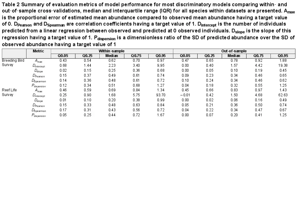
Table 2 Summary of evaluation metrics of model performance for most discriminatory models comparing within‐ and out‐of‐sample cross‐validations, median and interquartile range (IQR) for all species within datasets are presented. Amae is the proportional error of estimated mean abundance compared to observed mean abundance having a target value of 0. DPearson and DSpearman are correlation coefficients having a target value of 1. Dintercept is the number of individuals predicted from a linear regression between observed and predicted at 0 observed individuals. Dslope is the slope of this regression having a target value of 1. Pdispersion is a dimensionless ratio of the SD of predicted abundance over the SD of observed abundance having a target value of 1
Predictions of abundance from optimal models had a high correspondence with observed abundances, on average across all species, in both fish and birds (Fig. 4). However, as indicated by the evaluation metrics, the overall relationship was biased to be shallower than a 1:1 correspondence between observed and predicted abundance by models consistently overestimating low abundance and underestimating high abundances (Fig. 4; see the Supporting information for breakdown across individual optimal models). Applying a rescaling correction (rescaling‐predicted abundances to the observed abundance range) for each species helped to correct this systematic bias. Model performance improved as indicated by Dslope (before correction = 0.20–0.25 to after correction = 0.50–0.56) and Pdispersion (0.44–0.51 to 1.10); however, performance decreased when indicated by Dintercept (1.7–2.2 to 5.6–5.9) and Amae (0.64–0.69 to 0.88–0.94; see full results in the Supporting information).
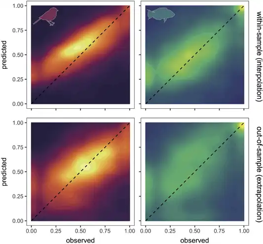
Figure 4
Contour plots of observed abundance versus model‐predicted abundance across Breeding Bird Survey and Real Life Survey datasets. Upper panels show within‐sample interpolation and lower panels show out‐of‐sample extrapolation of predicted values . Dashed line indicates 1:1 correspondence. Colour intensity indicates the number of records within contour. Both axes are log10+1 transformed and rescaled between 0 and 1 to show ability of models to discriminate abundance values. To avoid species with more data‐dominating patterns, for each species, we binned observations into 30 bins and estimated the mean predicted abundance for each observed abundance bin. Note that, due to the 0–1 transformation, a value of 0 is the minimum observed or predicted abundance value.
Model transferability to novel conditions (i.e. out‐of‐sample)
Transferring models to novel conditions, the best‐performing algorithm for each species in terms of discrimination (precision, accuracy) shifted to GLMs being the best for 33% species (27%, 39%), RF for 29% (40%, 20%), GAMs for 19% (19%, 17%) and GBM for 19% (15%, 24%) of the species (Fig. 2, Supporting information). Building models using abundance–absence data remained the best‐performing treatment of response data in terms of discrimination (precision, accuracy) for 60% (33%, 35%) of species, with 21% (41%, 38%) of species having best models when using only species abundances and 20% (26%, 27%) using a two‐step approach (Fig. 2).
Transferring models to novel conditions reduced model performance for most metrics across both birds and fishes (Table 2, Fig. 3). The general discrimination of high and low abundances remained (median DSpearman was 0.34 for birds and 0.34 for fishes). Dslope declined by more than half compared to within‐sample cross‐validations (median Dslope was 0.10 for birds and 0.06 for fishes). Accuracy also decreased compared to within‐sample cross‐validations, with a median of 0.78 and 0.83 in birds and fishes, respectively.
Predicted abundance still corresponded with observed abundances on average across all species, in both fishes and birds (Fig. 4), despite the poorer model performance. However, similar issues with a biased intercept and slope exist in the out‐of‐sample cross‐validations as for the within‐sample cross‐validations and were similarly corrected for by the rescaling procedure (Fig. 4; see the Supporting information for breakdown across individual optimal models and for comparisons with rescaling).
Species and data characteristics
The variation in model performance explained by species and data characteristics varied among performance metrics and was higher in general for within‐sample (R2 = 0.04–0.44) compared to out‐of‐sample cross‐validations (R2 = 0.01–0.33; Supporting information). All six evaluation metrics were affected by species or data characteristics in both birds and fishes (Supporting information). Pintercept had the most variation explained by species and data characteristics in both birds and fishes (R2 of 0.42–0.44).
We present the example metric DSpearman, which had an R2 between 0.16 and 0.33. The effects of species and data characteristics on DSpearman were highly consistent across within‐ and out‐of‐sample predictions and across both datasets (Fig. 5, Supporting information). More observations decreased the DSpearman. Higher frequency of occurrence increased DSpearman but only if species also had high number of observations. Species with higher abundance had higher DSpearman only if species had high frequency too. This last effect was not evident for fish species in out‐of‐sample predictions. Phylogenetic signal (Pagel's λ) in the residuals was very weak ranging from 0 to 0.17.

Figure 5
Effect of species and data characteristics on DSpearman for Breeding Bird Survey (a–c) and Reef Life Survey (d–f). Plots display marginal effects from multiple regressions fitted using phylogenetic generalised least squares for within‐sample cross‐validations. Lines represent mean predicted values. Shaded areas show uncertainty as mean ± (SE × 1.96) of coefficient values. All effects are significant at an alpha of 0.05, and interaction terms are only shown when significant. Full statistical results across all metrics, datasets and cross‐validations are displayed in the Supporting information. See the Supporting information for effect of species and data characteristics on DSpearman in out‐of‐sample predictions.
Discussion
We demonstrate the capacity to predict spatial patterns in abundance for many species if an appropriate model framework is chosen. The predictability of abundance using only the environmental response shapes of species has probably been under‐appreciated somewhat, in part due to many options for statistical models and only a few providing acceptable predictions. For example, using GAMs and GLMs, Johnston et al. () found a low rank correlation of 0.19 for predicted and observed seabird densities and therefore focused on coarser spatial scales for predictive analyses (see also Illan et al. ). Our results support that correlative abundance models could have an important role in quantifying the changing spatial patterns of species abundance due to environmental change, although many challenges remain. Here, we discuss our relative success and challenges in modelling abundance to better guide future applications.
Successful aspects of species abundance models
A small number of good approaches for predicting species abundance emerged after exploring a large set of models. Correlation values from our optimal models were higher than ~0.3 for more than 75% of species and higher than ~0.6 for 25% of species (Table 2). Our finding that RF perform well at within‐sample prediction provides solid evidence that specific case studies reporting similar results, such as in Balearic shearwaters Puffinus mauretanicus (Oppel et al. ), apply more generally, at least across the 800 species of bird and fish tested here. The high discrimination, precision and accuracy of RF would improve confidence in assigning regions as important abundance‐priority areas for conservation.
A focus on linear functions relating environments to local abundances may have previously reduced predictive performance. More flexible response curves of machine‐learning approaches allow for what may often be highly nonlinear abundance niche shapes (Pearce and Ferrier , Potts and Elith , Renwick et al. , Betts et al. ). Further optimised algorithms and deep learning approaches may better integrate abundance into biodiversity indicator frameworks, given the much better performance of machine‐learning approaches here (Jetz et al. ). If abundance has been perceived to be poorly explained by climate or other variables in the past, it could be falsely concluded that broad‐scale variables only weakly affect abundance and that abundance niches are more strongly constrained by factors other than species fundamental niches (but see Illan et al. , Dallas and Santini ).
Accurate prediction of local abundances with abiotic variables supports the theoretical prediction that fitness optima along abiotic niche axes filters down to determine ecologically successful locations of high population growth rates (Maguire ). The prediction of abundance from abiotic niche axes has been questioned by recent empirical studies (Dallas and Hastings , Santini et al. , Sporbert et al. ). These studies determine environmental effects on abundance indirectly from habitat suitability or environmental centroids. Here, we directly relate abundance to environmental conditions which provides a more direct quantification of species abundance niche with fewer assumptions (Osorio‐Olvera et al. ).
Modelling abundance directly was better than an indirect approach (i.e. comparing our abundance–absence models to two‐stage models) for more than 80% of species. This finding indicates that spatial abundance and occurrence patterns are somewhat mismatched or at least not always congruent (although it is challenging to completely disentangle abundance from occurrence, and vice versa). Mismatches arise from different ecological controls of abundance and occurrence, such as different demographic rates controlling each to different extents (McGill , Johnston et al. , Acevedo et al. , Bohner and Diez , Dallas and Santini , Schulz et al. , Yancovitch Shalom et al. ). Understanding such mismatches offers an important avenue for better understanding range and abundance shifts under climate change (Geppert et al. ) and potentially guiding spatial management and conservation. For example, a focus on occurrence can miss critical patches of high abundance driven by a few isolated factors (Johnston et al. , Suggitt et al. ). Such ‘strongholds' for species could be a common feature of ecological communities. Moving species distribution models beyond modelling occurrences, to help identify such areas, will require improving knowledge of species responses to environmental gradients using multiple performance metrics (i.e. occurrence, abundance, demographic rates) (Ehrlén and Morris , Ashcroft et al. , Bohner and Diez ).
Current limitations and challenges in species abundance models
We identify two important challenges in abundance models here. First, we systematically over‐predict low observed abundances and under‐predict high observed abundances (Pearce and Ferrier , Fukaya et al. , Ploton et al. ). Second, having more observations led to lower discrimination between high abundance sites and low abundance sites. These issues may jointly arise as we undoubtedly miss key biotic (e.g. ecological interactions) and microclimatic variables from our models (Lembrechts et al. ), leading to unexplained extreme local abundances.
Missing inter‐ and intraspecific interactions has been a well‐recognised problem in predictive occurrence‐based species distribution modelling (Guisan and Thuiller , Wisz et al. , Mouquet et al. , Pollock et al. ). For abundance‐based models, species interactions can drive population feedbacks that may be important for explaining extreme abundances, but are missing from models in general, leading to poor predictive performance. Recent theoretical work highlights how interaction feedbacks can modify abundance along environmental gradients, even if the fundamental niche shape is unimodal (Kéfi et al. , Liautaud et al. ). In addition, behavioural aggregations from seasonal migrations or resource booms can lead to extreme abundances, challenging the identification of appropriate statistical response distributions (Lindén and Mäntyniemi ). These points emphasise the need to better understand how local environments, individual behaviour and species interactions together shape macroecological abundance patterns. Novel joint species distribution modelling approaches (Ovaskainen et al. ), or direct estimation of interaction strengths (Wootton and Emmerson ) are promising tools to help address such questions.
Abundance‐based species distribution models could be further improved by considering fine‐scale microclimatic data, a concept gaining traction for occurrence‐based species distribution models (Potter et al. , Bennie et al. , Lembrechts et al. ) and critical for better conservation planning in the face of climate change (Roslin et al. , Isaak et al. ). Microclimate variation within grid cells can arise from variations in topography, aspect (Bennie et al. , Graae et al. ) and land‐use features (Chen et al. , , Zhao et al. , Senior et al. ) that filter species locally, and affect abundances, depending on species physiological and climatic niches (Ashcroft et al. , Nowakowski et al. , Waldock et al. ). Including fine‐scale temporal variability of environmental predictors may also improve model performances by better representing the duration and timing of key life‐history events that influence population dynamics (Supporting information; Andrew and Fox , Perez‐Navarro et al. ).
Incorporating environmental variation at the appropriate spatiotemporal scale for a given species is a critical area for model improvements (Roslin et al. , Ashcroft et al. , Rebaudo et al. ), especially for projections of future climate effects on species occurrence and abundance (Gillingham et al. , Hannah et al. , Maclean et al. , Woods et al. ). Our sensitivity analysis indicates improved model fit with improved data resolution for some species, but not all, when using just one year of BBS data linked to a finer temporal resolution of climate data (Supporting information). This finding indicates species‐specific behaviour (migratory versus non‐migratory), mobility (sedentary or mobile, home‐range size), life‐cycle (hibernators versus year‐round activity) and environmental niche characteristics (breadth, plasticity) could contribute to the resolution and windows of microclimatic data required to accurately estimate local abundances and occurrence (Bennie et al. , Lembrechts et al. ).
An additional problem, not present in occurrence‐based models, is that the probability of sampling a system in an extreme abundance state is higher with more samples, leading to outlier points (i.e. bright spots or dark spots). Perhaps these outliers could be an avenue to unveil important predictors of locations of hyper‐abundance or bright spots which in turn can comprise important targets for conservation (Cinner et al. , Frei et al. ). Biased predictions and unexplained outliers have important consequences. For example, the shallower slope of predicted versus observed abundance will underestimate change in abundance when the environment changes. In contrast, the likelihood of persistence will be overestimated because abundance losses in the last stages of population decline are poorly captured by models such as ours (Bates et al. ). As such, separate models for occurrence and abundance patterns will need to be calibrated and outputs combined. For occurrence‐based models, more data generally leads to better models (Chefaoui et al. ), and we identify the opposite here with the consequence that for abundance‐based models, data‐poor species perhaps generate overconfident models, a caveat worth exploring further.
We identify that the transferability of species abundance models to novel environmental conditions is presently limited. This shortcoming also applies to occurrence‐based species distribution models (Sequeira et al. , Yates et al. ) and models of family‐level abundances (Sequeira et al. ) but may be exacerbated when considering species abundance. Models with perfect discrimination of presence–absence can still have poor predictive power of abundance values because more mechanisms underlie abundance variation, and errors in capturing each mechanism using statistical response functions will accumulate (Bahn and McGill , Johnston et al. ). We demonstrate model performance also declines when predicting outside the bounds of even a single covariate (rather than a spatial block (Ploton et al. )), with strong consequences for future climatic predictions.
Novel climatic conditions are fast emerging (Williams and Jackson ) and hence solutions that improve model transferability are urgently needed (Radeloff et al. , Harris et al. ). Whilst mechanistic models offer accurate predictions at coarse spatial scales (Fernandes et al. , ), further integration with correlative frameworks may enable prediction at fine scales and in novel environments (Cheung et al. , Fernandes et al. , Gamliel et al. ).
Which species to target for abundance‐based species distribution modelling?
Our consideration of strengths and limitations of species abundance models can help guide their application for predicting the spatial distribution of species abundance for systematic conservation planning (Margules and Pressey , Pinsky et al. , Pollock et al. ). Importantly, from a conservation perspective, we outline how model performance relates to rarity and thus extinction risk. Our results suggest that species with low frequency of occurrence and low mean abundance will be more challenging to predict. Perhaps such species are only weakly constrained by physiological niche limits and more strongly constrained by meta‐population dispersal, microclimate effects and availability of resources, hosts or prey items (Selig et al. , Venter et al. , Mouillot et al. , Suggitt et al. ). In contrast, common and abundant species that mostly contribute to ecosystem functions and services may be good targets for species abundance modelling (Winfree et al. , Mouillot et al. ). We also highlight how the treatment of abundance data can modify how well models perform in accuracy, discrimination and precision, which could have important consequences depending on the target application. Here, consideration of species abundances as well as changes in occurrence should greatly assist understanding how biodiversity change affects ecosystem functioning and human well‐being (Johnston et al. , Kissling et al. , Pinsky et al. ).
Conclusions
Species abundances in localised field surveys can be predicted for a large number of species on the basis of broad‐scale environmental and human factors, such as climate, land cover and habitat area. Species abundance models showed surprisingly similar performance for species from two very different taxonomic groups and ecological contexts. Transferring models to novel conditions was very challenging, however. Models fitted better for more frequently encountered and abundant species, highlighting that abundance models may be most applicable to questions relating to ecosystem function and service provision rather than in modelling rare or endemic species under extinction threats. When common species are to be prioritised (Pinsky et al. ), species abundance models could be used in many ways, providing spatial maps of species abundance, landscape scale estimates of ecological processes and services (Gilby et al. ) or helping to identify regions with large, stable, viable populations that can act as sources and facilitate reserve spillover and ecosystem stability (Halpern et al. , Rondinini and Chiozza , Timus et al. , Cabral et al. ; Table 1). We argue that spatial abundance models can provide critical biodiversity information with the potential to improve the ecological relevance and species conservation applications of species distribution models.
Acknowledgements
– We thank the many Reef Life Survey (RLS) divers who participated in data collection and provided ongoing expertise and commitment to the program. We thank the North American Breeding Bird Survey Dataset for providing access to the data and the thousands of participants who annually perform and coordinate the survey. CW was supported by the BiodivERsA grant Reef‐Futures (SNF_184118). JT acknowledges Research Council of Norway‐funded project BiodivERsA (Reef‐Futures, no. 295340). WWLC acknowledges funding support from the Natural Sciences and Engineering Research Council of Canada for the BiodivERsA project Reef‐Futures. Reef Life Survey uses the NCRIS‐enabled Integrated Marine Observing System (IMOS) infrastructure for database support and storage, with support from Antonia Cooper and Elizabeth Oh. Thanks for IT and server support from Dominic Michel, Hussain Abbas and Benjamin Flück. Thanks to ‘Reef‐Futures' workshop attendees who provided constructive feedback on this work in addition to Jonathan Chase and Valentin Verdon who provided valuable feedback on previous manuscript drafts.
Funding
– CW and JT supported by BiodivERsA Reef‐Futures no. 295340.
Author contributions
Conor Waldock: Conceptualization (lead); Data curation (lead); Formal analysis (lead); Investigation (lead); Methodology (lead); Software (lead); Validation (lead); Visualization (lead); Writing – original draft (lead); Writing – review and editing (lead). Rick D. Stuart‐Smith: Data curation (equal); Writing – review and editing (equal). Camille Albouy: Funding acquisition (equal); Writing – review and editing (equal). William W. L. Cheung: Writing – review and editing (equal). Graham J. Edgar: Data curation (equal); Writing – review and editing (equal). David Mouillot: Funding acquisition (equal); Writing – review and editing (equal). Jerry Tjiputra: Data curation (equal); Writing – review and editing (equal). Loic Pellissier: Funding acquisition (equal); Supervision (equal); Writing – review and editing (equal).
Transparent Peer Review
The peer review history for this article is available at <https://publons.com/publon/10.1111/ecog.05694>.
Supporting information
The supporting information associated with this article is available from the online version.
References
- Acevedo P. et al. 2017. Population dynamics affect the capacity of species distribution models to predict species abundance on a local scale. – Divers. Distrib. 23: 1008–1017.
- Andrew M. E. and Fox E. 2020. Modelling species distributions in dynamic landscapes: the importance of the temporal dimension. – J. Biogeogr. 47: 1510–1529.
- Antão L. H. et al. 2020a. Contrasting latitudinal patterns in diversity and stability in a high‐latitude species‐rich moth community. – Global Ecol. Biogeogr. 29: 896–907.
- Antão L. H. et al. 2020b. Temperature‐related biodiversity change across temperate marine and terrestrial systems. – Nat. Ecol. Evol. 4: 927–933.
- Ashcroft M. B. et al. 2014. Testing the ability of topoclimatic grids of extreme temperatures to explain the distribution of the endangered brush‐tailed rock‐wallaby Petrogale penicillata. – J. Biogeogr. 41: 1402–1413.
- Ashcroft M. B. et al. 2017. Moving beyond presence and absence when examining changes in species distributions. – Global Change Biol. 23: 2929–2940.
- Austin M. P. 2002. Spatial prediction of species distribution: an interface between ecological theory and statistical modelling. – Ecol. Model. 157: 101–118.
- Bahn V. and McGill B. J. 2013. Testing the predictive performance of distribution models. – Oikos 122: 321–331.
- Bates A. E. et al. 2014. Defining and observing stages of climate‐mediated range shifts in marine systems. – Global Environ. Change 26: 27–38.
- Bates A. E. et al. 2015. Distinguishing geographical range shifts from artefacts of detectability and sampling effort. – Divers. Distrib. 21: 13–22.
- Becker E. A. et al. 2019. Predicting cetacean abundance and distribution in a changing climate. – Divers. Distrib. 25: 626–643.
- Bennie J. et al. 2008. Slope, aspect and climate: spatially explicit and implicit models of topographic microclimate in chalk grassland. – Ecol. Model. 216: 47–59.
- Bennie J. et al. 2014. Seeing the woods for the trees – when is microclimate important in species distribution models? – Global Change Biol. 20: 2699–2700.
- Betts M. G. et al. 2019. Synergistic effects of climate and land‐cover change on long‐term bird population trends of the western USA: a test of modeled predictions. – Front. Ecol. Evol. 7: 186.
- Blomberg S. P. and Symonds M. R. E. 2014. Modern phylogenetic comparative methods and their application in evolutionary biology. – Springer.
- Bohner T. and Diez J. 2020. Extensive mismatches between species distributions and performance and their relationship to functional traits – Ecol. Lett. 23: 33–44.
- Boucher‐Lalonde V. et al. 2012. How are tree species distributed in climatic space? A simple and general pattern. – Global Ecol. Biogeogr. 21: 1157–1166.
- Bowler D. E. et al. 2017. Cross‐taxa generalities in the relationship between population abundance and ambient temperatures. – Proc. R. Soc. B 284: 20170870.
- Breiman L. 2001. Random forests. – Mach. Learn. 45: 5–32.
- Brown J. et al. 1995. Spatial variation in abundance. – Ecology 76: 2028–2043.
- Brun P. et al. 2020. Model complexity affects species distribution projections under climate change. – J. Biogeogr. 47: 130–142.
- Burnham K. P. and Anderson D. R. 2002. Model selection and multimodel inference: a practical information–theoretic approach. – Springer.
- Cabral R. B. et al. 2020. A global network of marine protected areas for food. – Proc. Natl Acad. Sci. USA 117: 28134–28139.
- Ceballos G. et al. 2020. Vertebrates on the brink as indicators of biological annihilation and the sixth mass extinction. – Proc. Natl Acad. Sci. USA 117: 13596–13602.
- Chefaoui R. M. et al. 2011. Effects of species' traits and data characteristics on distribution models of threatened invertebrates. – Anim. Biodivers. Conserv. 34: 229–247.
- Chen J. et al. 1999. Microclimate in forest ecosystem and landscape ecology: variations in local climate can be used to monitor and compare the effects of different management regimes. – Bioscience 49: 288–297.
- Chen X. et al. 2006. Remote sensing image‐based analysis of the relationship between urban heat island and land use/cover changes. – Remove Sens. Environ. 104: 133–146.
- Cheung W. W. L. et al. 2008. Modelling present and climate‐shifted distributions of marine fishes and invertebrates. – Fish. Cent. Res. Rep. 16: 72.
- Chisholm R. A. and Muller‐Landau H. C. 2011. A theoretical model linking interspecific variation in density dependence to species abundances. – Theor. Ecol. 4: 241–253.
- Chu C. et al. 2016. Direct effects dominate responses to climate perturbations in grassland plant communities. – Nat. Commun. 7: 1–10.
- Cinner J. et al. 2016. Bright spots among the world's coral reefs. – Nature 535: 416–419.
- Clements C. F. et al. 2017. Body size shifts and early warning signals precede the historic collapse of whale stocks. – Nat. Ecol. Evol. 1: 1–6.
- Cresswell A. K. et al. 2017. Translating local benthic community structure to national biogenic reef habitat types. – Global Ecol. Biogeogr. 26: 1112–1125.
- Cruz‐Cárdenas G. et al. 2014. Potential species distribution modeling and the use of principal component analysis as predictor variables. – Rev. Mex. Biodivers. 85: 189–199.
- Dallas T. A. and Hastings A. 2018. Habitat suitability estimated by niche models is largely unrelated to species abundance. – Global Ecol. Biogeogr. 27: 1448–1456.
- Dallas T. A. and Santini L. 2020. The influence of stochasticity, landscape structure and species traits on abundant–centre relationships. – Ecography 43: 1341–1351.
- Dallas T. et al. 2017. Species are not most abundant in the centre of their geographic range or climatic niche. – Ecol. Lett. 20: 1526–1533.
- De Marco P. and Nóbrega C. C. 2018. Evaluating collinearity effects on species distribution models: an approach based on virtual species simulation. – PLoS One 13: e0202403.
- Denes F. V et al. 2015. Estimating abundance of unmarked animal populations: accounting for imperfect detection and other sources of zero inflation. – Methods Ecol. Evol. 6: 543–556.
- Edgar G. J. and Stuart‐Smith R. D. 2014. Systematic global assessment of reef fish communities by the Reef Life Survey program. – Sci. Data 1: 140007.
- Ehrlén J. and Morris W. F. 2015. Predicting changes in the distribution and abundance of species under environmental change. – Ecol. Lett. 18: 303–314.
- Evans M. R. 2012. Modelling ecological systems in a changing world. – Phil. Trans. R. Soc. B 367: 181–190.
- Fei S. et al. 2017. Divergence of species responses to climate change. – Sci. Adv. 3: e1603055.
- Fernandes J. A. et al. 2013. Modelling the effects of climate change on the distribution and production of marine fishes: accounting for trophic interactions in a dynamic bioclimate envelope model. – Global Change Biol. 19: 2596–2607.
- Fernandes J. A. et al. 2020. Can we project changes in fish abundance and distribution in response to climate? – Global Change Biol. 26: 3891–3905.
- Flores C. E. et al. 2018. Spatial abundance models and seasonal distribution for guanaco Lama guanicoe in central Tierra del Fuego, Argentina. – PLoS One 13(5): e0197814.
- Frei B. et al. 2018. Bright spots in agricultural landscapes: identifying areas exceeding expectations for multifunctionality and biodiversity. – J. Appl. Ecol. 55: 2731–2743.
- Friedman J. H. 2001. Greedy function approximation: a gradient boosting machine. – Ann. Stat. 29: 1189–1232.
- Fukaya K. et al. 2020. Integrating multiple sources of ecological data to unveil macroscale species abundance. – Nat. Commun. 11: 1695.
- Gamliel I. et al. 2020. Incorporating physiology into species distribution models moderates the projected impact of warming on selected Mediterranean marine species. – Ecography 43: 1090–1106.
- Genung M. A. et al. 2020. Species loss drives ecosystem function in experiments, but in nature the importance of species loss depends on dominance. – Global Ecol. Biogeogr. 29: 1531–1541.
- Geppert C. et al. 2020. Consistent population declines but idiosyncratic range shifts in Alpine orchids under global change. – Nat. Commun. 11: 5835.
- Gilby B. L. et al. 2020. Identifying restoration hotspots that deliver multiple ecological benefits. – Restor. Ecol. 28: 222–232.
- Gillingham P. K. et al. 2012. The effect of spatial resolution on projected responses to climate warming. – Divers. Distrib. 18: 990–1000.
- Graae B. J. et al. 2018. Stay or go – how topographic complexity influences alpine plant population and community responses to climate change. – Perspect. Plant Ecol. Evol. Syst. 30: 41–50.
- Guillera‐Arroita G. 2017. Modelling of species distributions, range dynamics and communities under imperfect detection: advances, challenges and opportunities. – Ecography 40: 281–295.
- Guisan A. and Thuiller W. 2005. Predicting species distribution: offering more than simple habitat models. – Ecol. Lett. 8: 993–1009.
- Hallett L. M. et al. 2018. Tradeoffs in demographic mechanisms underlie differences in species abundance and stability. – Nat. Commun. 9: 1–6.
- Halpern B. S. et al. 2010. Spillover from marine reserves and the replenishment of fished stocks. – Environ. Conserv. 36: 268–276.
- Hannah L. et al. 2014. Fine‐grain modeling of species' response to climate change: holdouts, stepping‐stones and microrefugia. – Trends Ecol. Evol. 29: 390–397.
- Harris R. M. B. et al. 2018. Biological responses to the press and pulse of climate trends and extreme events. – Nat. Clim. Change 8: 579–587.
- Hastings R. A. et al. 2020. Climate change drives poleward increases and equatorward declines in marine species. – Curr. Biol. 30: 1572.e2–1577.e2.
- Holt R. D. 2009. Bringing the Hutchinsonian niche into the 21st century: ecological and evolutionary perspectives. – Proc. Natl Acad. Sci. USA 106: 19659–19665.
- Holt R. D. 2020. Reflections on niches and numbers. – Ecography 43: 387–390.
- Hutchings J. A. and Reynolds J. D. 2004. Marine fish population collapses: consequences for recovery and extinction risk. – Bioscience 54: 297.
- Illan J. G. et al. 2014. Precipitation and winter temperature predict long‐term range‐scale abundance changes in western North American birds. – Global Change Biol. 20: 3351–3364.
- Isaak D. J. et al. 2017. Big biology meets microclimatology: defining thermal niches of ectotherms at landscape scales for conservation planning. – Ecol. Appl. 27: 977–990.
- Jetz W. et al. 2012. The global diversity of birds in space and time. – Nature 491: 444–448.
- Jetz W. et al. 2014. Global distribution and conservation of evolutionary distinctness in birds. – Curr. Biol. 24: 919–930.
- Jetz W. et al. 2019. Essential biodiversity variables for mapping and monitoring species populations. – Nat. Ecol. Evol. 3: 539–551.
- Johnston A. et al. 2013. Observed and predicted effects of climate change on species abundance in protected areas. – Nat. Clim. Change 3: 1055–1061.
- Johnston A. et al. 2015. Abundance models improve spatial and temporal prioritization of conservation resources. – Ecol. Appl. 25: 1749–1756.
- Kallasvuo M. et al. 2017. Modeling the spatial distribution of larval fish abundance provides essential information for management. – Can. J. Fish. Aquat. Sci. 74: 636–649.
- Kéfi S. et al. 2016. When can positive interactions cause alternative stable states in ecosystems? – Funct. Ecol. 30: 88–97.
- Kissling W. D. et al. 2018. Building essential biodiversity variables (EBVs) of species distribution and abundance at a global scale. – Biol. Rev. 93: 600–625.
- Lembrechts J. J. et al. 2019. Incorporating microclimate into species distribution models. – Ecography 42: 1267–1279.
- Lenoir J. and Svenning J.‐C. 2013. Latitudinal and elevational range shifts under contemporary climate change. – Encycl. Biodivers. 4: 599–611.
- Lenoir J. et al. 2020. Species better track climate warming in the oceans than on land. – Nat. Ecol. Evol. 4: 1044–1059.
- Liautaud K. et al. 2019. Superorganisms or loose collections of species? A unifying theory of community patterns along environmental gradients. – Ecol. Lett. 22: ele.13289.
- Lindén A. and Mäntyniemi S. 2011. Using the negative binomial distribution to model overdispersion in ecological count data. – Ecology 92: 1414–1421.
- Maclean I. M. D. et al. 2015. Microclimates buffer the responses of plant communities to climate change. – Global Ecol. Biogeogr. 24: 1340–1350.
- Maguire B. 1973. Niche response structure and the analytical potentials of its relationship to the habitat. – Am. Nat. 107: 213–246.
- Margules C. R. and Pressey R. L. 2000. Systematic conservation planning. – Nature 405: 243–253.
- Martínez‐Meyer E. et al. 2013. Ecological niche structure and rangewide abundance patterns of species. – Biol. Lett. 9: 20120637.
- Matías L. et al. 2019. Disentangling the climatic and biotic factors driving changes in the dynamics of Quercus suber populations across the species' latitudinal range. – Divers. Distrib. 25: 524–535.
- Maxwell S. L. et al. 2019. Conservation implications of ecological responses to extreme weather and climate events. – Divers. Distrib. 25: 613–625.
- McGill B. J. 2012. Trees are rarely most abundant where they grow best. – J. Plant Ecol. 5: 46–51.
- McPherson J. and Jetz W. 2007. Effects of species? Ecology on the accuracy of distribution models. – Ecography 30: 135–151.
- Merow C. et al. 2014. What do we gain from simplicity versus complexity in species distribution models? – Ecography 37: 1267–1281.
- Meynard C. N. et al. 2019. Testing methods in species distribution modelling using virtual species: what have we learnt and what are we missing? – Ecography 42: 2021–2036.
- Mi C. et al. 2017. Combining occurrence and abundance distribution models for the conservation of the great bustard. – PeerJ 5: e4160.
- Morrissey M. B. and Ruxton G. D. 2018. Multiple regression is not multiple regressions: the meaning of multiple regression and the non‐problem of collinearity. – Phil. Theory Pract. Biol. 10: 2–24.
- Mouillot D. et al. 2016. Global marine protected areas do not secure the evolutionary history of tropical corals and fishes. – Nat. Commun. 7: 10359.
- Mouquet N. et al. 2015. Predictive ecology in a changing world. – J. Appl. Ecol. 52: 1293–1310.
- Newbold T. et al. 2009. Effect of characteristics of butterfly species on the accuracy of distribution models in an arid environment. – Biodivers. Conserv. 18: 3629–3641.
- Norberg A. et al. 2019. A comprehensive evaluation of predictive performance of 33 species distribution models at species and community levels. – Ecol. Monogr. 89: e01370.
- Nowakowski A. J. et al. 2018. Thermal biology mediates responses of amphibians and reptiles to habitat modification. – Ecol. Lett. 21: 345–355.
- Oppel S. et al. 2012. Comparison of five modelling techniques to predict the spatial distribution and abundance of seabirds. – Biol. Conserv. 156: 94–104.
- Osorio‐Olvera L. et al. 2019. On population abundance and niche structure. – Ecography 42: 1415–1425.
- Osorio‐Olvera L. et al. 2020. Relationships between population densities and niche‐centroid distances in North American birds. – Ecol. Lett. 23: 555–564.
- Ovaskainen O. et al. 2017. How to make more out of community data? A conceptual framework and its implementation as models and software. – Ecol. Lett. 20: 561–576.
- Pardieck K. L. et al. 2019. North American Breeding Bird Survey Dataset 1966–2018, ver. 2018.0. – U.S. Geological Survey, Patuxent Wildlife Research Center.
- Pauly D. and Froese R. 2010. A count in the dark. – Nat. Geosci. 3: 662–663.
- Pearce J. and Ferrier S. 2001. The practical value of modelling relative abundance of species for regional conservation planning: a case study. – Biol. Conserv. 98: 33–43.
- Pearce‐Higgins J. W. et al. 2015. Geographical variation in species' population responses to changes in temperature and precipitation. – Proc. R. Soc. B 282: 20151561.
- Pereira H. M. et al. 2013. Essential biodiversity variables. – Science 339: 277–278.
- Perez‐Navarro M. A. et al. 2021. Temporal variability is key to modelling the climatic niche. – Divers. Distrib. 27: 473–484.
- Peterson A. T. et al. 2011. Ecology niches and geographic distributions. – Princeton Univ. Press.
- Pinsky M. L. et al. 2020. Ocean planning for species on the move provides substantial benefits and requires few tradeoffs. – Sci. Adv. 6: eabb8428.
- Ploton P. et al. 2020. Spatial validation reveals poor predictive performance of large‐scale ecological mapping models. – Nat. Commun. 11: 4540.
- Pollock L. J. et al. 2020. Protecting biodiversity (in all its complexity): new models and methods. – Trends Ecol. Evol. 35: 1119–1128.
- Potter K. A. et al. 2013. Microclimatic challenges in global change biology. – Global Change Biol. 19: 2932–2939.
- Potts J. M. and Elith J. 2006. Comparing species abundance models. – Ecol. Model. 199: 153–163.
- Purvis A. et al. 2000. Predicting extinction risk in declining species. – Proc. R. Soc. B 267: 1947–1952.
- Rabosky D. L. et al. 2018. An inverse latitudinal gradient in speciation rate for marine fishes. – Nature 559: 392–395.
- Radeloff V. C. et al. 2015. The rise of novelty in ecosystems. – Ecol. Appl. 25: 2051–2068.
- Randin C. F. et al. 2006. Are niche‐based species distribution models transferable in space? – J. Biogeogr. 33: 1689–1703.
- Ready J. et al. 2010. Predicting the distributions of marine organisms at the global scale. – Ecol. Model. 221: 467–478.
- Rebaudo F. et al. 2016. Microclimate data improve predictions of insect abundance models based on calibrated spatiotemporal temperatures. – Front. Physiol. 7: 139.
- Renwick A. R. et al. 2012. Modelling changes in species' abundance in response to projected climate change. – Divers. Distrib. 18: 121–132.
- Ricart A. M. et al. 2018. Long‐term shifts in the north western Mediterranean coastal seascape: the habitat‐forming seaweed Codium vermilara. – Mar. Pollut. Bull. 127: 334–341.
- Roberts D. R. et al. 2017. Cross‐validation strategies for data with temporal, spatial, hierarchical or phylogenetic structure. – Ecography 40: 913–929.
- Román‐Palacios C. and Wiens J. J. 2020. Recent responses to climate change reveal the drivers of species extinction and survival. – Proc. Natl Acad. Sci. USA 117: 4211–4217.
- Rondinini C. and Chiozza F. 2010. Quantitative methods for defining percentage area targets for habitat types in conservation planning. – Biol. Conserv. 143: 1646–1653.
- Roslin T. et al. 2009. Some like it hot: microclimatic variation affects the abundance and movements of a critically endangered dung beetle. – Insect Conserv. Divers. 2: 232–241.
- Santini L. et al. 2019. Addressing common pitfalls does not provide more support to geographical and ecological abundant‐centre hypotheses. – Ecography 42: 696–705.
- Schulz T. et al. 2020. Long‐term demographic surveys reveal a consistent relationship between average occupancy and abundance within local populations of a butterfly metapopulation. – Ecography 43: 306–317.
- Selig E. R. et al. 2014. Global priorities for marine biodiversity conservation. – PLoS One 9: e82898.
- Senior R. A. et al. 2017. A pantropical analysis of the impacts of forest degradation and conversion on local temperature. – Ecol. Evol. 7: 7897–7908.
- Sequeira A. M. M. et al. 2018a. Transferring biodiversity models for conservation: opportunities and challenges. – Methods Ecol. Evol. 9: 1250–1264.
- Sequeira A. M. M. et al. 2018b. Challenges of transferring models of fish abundance between coral reefs. – PeerJ 6: e4566.
- Sherley R. B. et al. 2020. The conservation status and population decline of the African penguin deconstructed in space and time. – Ecol. Evol. 10: 8506–8516.
- Sporbert M. et al. 2020. Testing macroecological abundance patterns: the relationship between local abundance and range size, range position and climatic suitability among European vascular plants. – J. Biogeogr. 47: 2210–2222.
- Stacklies W. et al. 2007. pcaMethods ‐ a bioconductor package providing PCA methods for incomplete data. – Bioinformatics. 23: 1164–1167.
- Stuart‐Smith R. D. et al. 2013. Integrating abundance and functional traits reveals new global hotspots of fish diversity. – Nature 501: 539–542.
- Suggitt A. J. et al. 2018. Extinction risk from climate change is reduced by microclimatic buffering. – Nat. Clim. Change 8: 713–717.
- Thuiller W. et al. 2019. Uncertainty in ensembles of global biodiversity scenarios. – Nat. Commun. 10: 1446.
- Timus N. et al. 2017. Conservation implications of source‐sink dynamics within populations of endangered Maculinea butterflies. – J. Insect Conserv. 21: 369–378.
- Vanderwal J. et al. 2009. Abundance and the environmental niche: environmental suitability estimated from niche models predicts the upper limit of local abundance. – Am. Nat. 174: 282–291.
- Vázquez D. P. et al. 2007. Species abundance and asymmetric interaction strength in ecological networks. – Oikos 116: 1120–1127.
- Venter O. et al. 2014. Targeting global protected area expansion for imperiled biodiversity. – PLoS Biol. 12: e1001891.
- Violle C. et al. 2017. Functional rarity: the ecology of outliers. – Trends Ecol. Evol. 32: 356–367.
- Waldock C. et al. 2019. The shape of abundance distributions across temperature gradients in reef fishes. – Ecol. Lett. 22: 685–696.
- Waldock C. A. et al. 2020. Insect occurrence in agricultural land‐uses depends on realized niche and geographic range properties. – Ecography 43: 1717–1728.
- Williams J. W. and Jackson S. T. 2007. Novel climates, no‐analog communities and ecological surprises. – Front. Ecol. Environ. 5: 475–482.
- Williams R. et al. 2014. Prioritizing global marine mammal habitats using density maps in place of range maps. – Ecography 37: 212–220.
- Winfree R. et al. 2015. Abundance of common species, not species richness, drives delivery of a real‐world ecosystem service. – Ecol. Lett. 18: 626–635.
- Wisz M. S. et al. 2008. Effects of sample size on the performance of species distribution models. – Divers. Distrib. 14: 763–773.
- Wisz M. S. et al. 2013. The role of biotic interactions in shaping distributions and realised assemblages of species: Implications for species distribution modelling. – Biol. Rev. 88: 15–30.
- Woods H. A. et al. 2015. The roles of microclimatic diversity and of behavior in mediating the responses of ectotherms to climate change. – J. Therm. Biol. 54: 86–97.
- Wootton J. T. and Emmerson M. 2005. Measurement of interaction strength in nature. – Annu. Rev. Ecol. Evol. Syst. 36: 419–444.
- Yancovitch Shalom H. et al. 2020. A closer examination of the ‘abundant centre' hypothesis for reef fishes. – J. Biogeogr. 47: 2194–2209.
- Yañez‐Arenas C. et al. 2014. Predicting species' abundances from occurrence data: effects of sample size and bias. – Ecol. Model. 294: 36–41.
- Yates K. L. et al. 2018. Outstanding challenges in the transferability of ecological models. – Trends Ecol. Evol. 33: 790–802.
- Yenni G. et al. 2017. Do persistent rare species experience stronger negative frequency dependence than common species? – Global Ecol. Biogeogr. 26: 513–523.
- Yokomizo H. et al. 2009. Managing the impact of invasive species: the value of knowing the density–impact curve. – Ecol. Appl. 19: 376–386.
- Zhao L. et al. 2014. Strong contributions of local background climate to urban heat islands. – Nature 511: 216–219.
- Zurell D. et al. 2016. Benchmarking novel approaches for modelling species range dynamics. – Global Change Biol. 22: 2651–2664.